Week 10 - Validation studies of Symmetry BC vs Wedge BC in OpenFOAM vs Analytical H.P equation
AIM:
The objective of this study is to investigate the influence of the wedge angle and boundary conditions on the simulation of axisymmetric laminar flow within a cylindrical pipe.
THEORETICAL INTRODUCTION:
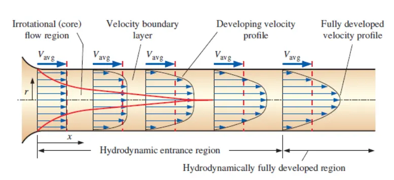
The image depicts two regions in a pipe: the hydrodynamic entrance region, where flow develops a velocity profile due to viscous forces, and the fully developed region, where flow characteristics become constant. The boundary layer, dividing the flow into irrotational and boundary layer regions, experiences significant velocity changes due to viscous effects. In the irrotational region, friction is negligible, and velocity remains essentially radial. The boundary layer thickness increases gradually until the mid-section, where the velocity profile becomes fully developed. This transition from entry to full development is termed the hydrodynamic entrance region, characterized by changing velocity profiles. In the fully developed flow region, velocity remains constant across the pipe, forming a parabolic profile. Shear stress is highest at the wall and lowest at the center due to its direct proportionality to the velocity gradient.
Axisymmetric Flow:
Axisymmetric flow occurs when the flow pattern remains identical in every plane passing through a specific straight line known as the symmetry axis. Each longitudinal plane through this axis exhibits an identical streamline pattern, contributing to a symmetrical fluid flow.
- Laminar Flow: In fluid dynamics, laminar flow is characterized by the orderly movement of fluid particles along smooth paths in layers. Each layer smoothly passes adjacent layers with minimal mixing. At lower velocities, laminar flow prevents lateral mixing, resembling the sliding of playing cards. There are no cross-currents perpendicular to the flow direction, and the absence of eddies or swirls defines the nature of laminar flow. This regime is marked by high momentum diffusion and low momentum convection.
When fluid traverses a closed channel like a pipe or between two flat plates, the flow type depends on velocity and viscosity. Laminar flow occurs at lower velocities, determined by the Reynolds number—a dimensionless parameter accounting for fluid velocity, viscosity, density, and channel dimensions. - Comparison between Turbulent and Laminar Flow:
The Reynolds number (Re) plays a crucial role in predicting flow patterns. Low Reynolds numbers favor laminar flow, characterized by sheet-like flow patterns, while high Reynolds numbers lead to turbulence. Turbulence arises from variations in fluid speed and direction, causing intersecting or counterflowing currents (eddy currents). This turbulence consumes energy and increases the risk of cavitation in liquids.
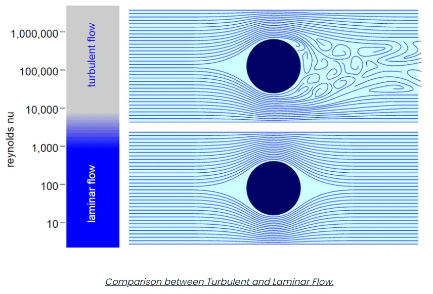
Reynolds numbers find application in diverse fluid mechanics scenarios, from predicting laminar-to-turbulent flow transitions to scaling effects in different-sized flow situations. Applications range from liquid flow in pipes to the airflow over aircraft wings. Predicting turbulence onset and scaling effects aids in understanding fluid behavior at various scales, impacting local and global air or water movements and associated meteorological and climatological effects.
HAGEN-POISEUILLE EQUATION:-
In non fluid dynamics the hagen-poiseuille equation is a physical law that gives the pressure drop in an incompressible and newtonian fluid in laminar flow flowing throught a long cylinder pipe of constant cross section.
The equations describes pressure drop as follows,
Piezo metric pressure drop, `gradp=(32*mu*V_(avg)*L*Lhydro)/d^2`
Wedge Boundary Conditions:
- Used in computational fluid dynamics to define an axisymmetric situation, such as a cylinder.
- Requires the model and flow to be axisymmetric along a central line.
- All physical variables of the flow must have the same value and distribution at a given radius for all angles.
- Specified by two planes on separate sides of the domain (front and back) along surfaces running along the axis.
- Applicable for 2D simulations only.
Symmetry Boundary Conditions:
- Defines a mirror face/surface in computational fluid dynamics.
- Should be used when the physical object or geometry and the expected flow field pattern are mirrored along that surface.
- Reduces the computational domain by essentially halving it, leading to faster solution times.
- Imposes constraints on flow variables: fluxes across the symmetry are zero, and normal components of all variables are set to zero.
- Can be applied to both planar or non-planar faces/surfaces on the domain boundaries.
METHODOLOGY:
For the numerical simulation conducted in the OpenFOAM software, an axisymmetric wedge domain was employed, and appropriate boundary conditions were applied to achieve accurate flow simulation while minimizing assumptions. This methodology aimed to emulate real-world fluid flow dynamics in a controlled environment.
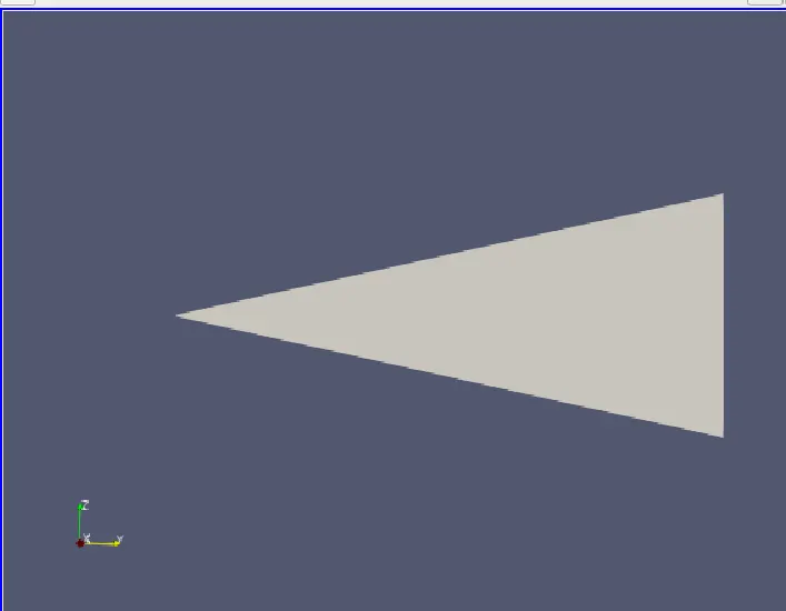
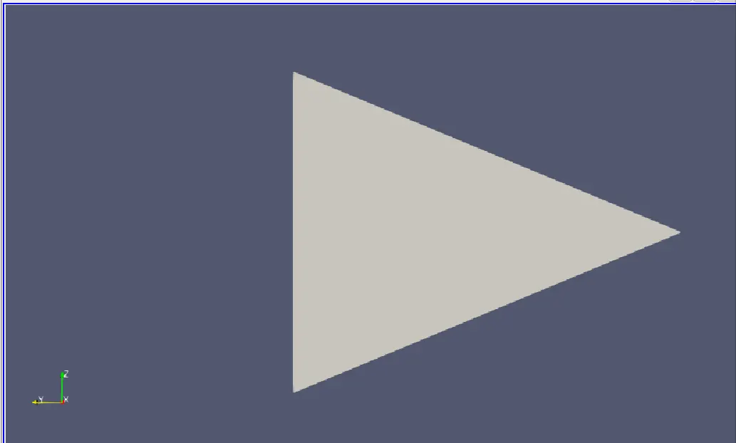
Lets consider the below image as reference to construct the wedge:
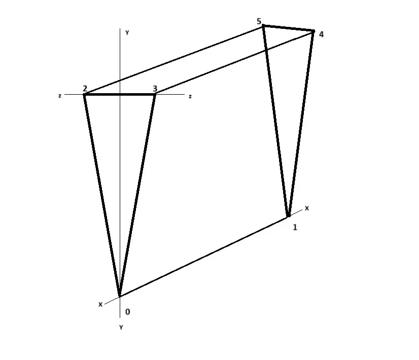
If the wedge length is 'Lpipe' and angle is 'theta'
then,
Diameter of the pipe in meters, d=0.015
Radius, r = d / 2
Angle of wedge, theta is variable (10, 25, 45)
Length of developing flow, Lhydro = 0.05 * Re * d=1.5750 m
Length of pipe, Lpipe = Lhydro + 0.1*Lhydro=1.7325 m
Coordinates of vertices of the wedge:
v0 = [0, 0, 0]
v1 = [Lpipe, 0, 0]
v2 = [0, r * cos(theta / 2), -r * sin(theta / 2)]
v3 = [0, r * cos(theta / 2), r * sin(theta / 2)]
v4 =[ Lpipe, r * cos(theta / 2), r * sin(theta / 2)]
v5 = [Lpipe, r * cos(theta / 2), -r * sin(theta / 2)]
Hagen–Poiseuille's law describes the pressure drop (ΔP) in an incompressible and Newtonian fluid flowing through a long cylindrical pipe with laminar flow and constant cross-section. The equation is expressed as:
`triangle p = (8 mu L Q)/( pi R ^4)`�=8�����4
where:
- ΔP is the pressure drop across the pipe,
- η is the dynamic viscosity of the fluid,
- L is the length of the pipe,
- Q is the volumetric flow rate of the fluid, and
- r is the radius of the pipe.
This equation highlights the relationship between the pressure drop, viscosity, length of the pipe, volumetric flow rate, and the fourth power of the radius of the pipe. It is essential for understanding the behavior of fluid flow in cylindrical pipes under laminar conditions. Keep in mind that this equation is applicable only when the flow is laminar and the fluid is Newtonian.
AUTOMATED CODE FOR HAGEN-POISEUILLE FLOW:
It can generate all necessary files required to do the simulation in OPEN-FOAM, that are re-arranged in the folders.
% Fluid flow in a pipe (Hagen-Poiseuille flow)
%code to automate generation of files for OPEN-FOAM

clear all
close all
clc

%The Renoylds number
Re=input('Enter value for Reynolds Number =');
%Diameter of the pipe in meters
d=input('Enter value of the pipe diameter = ');
%radius
r = d / 2;
%Angle of the wedge in degrees
theta= input('Enter value of the wedge angle = ');
%length of developing flow
Lhydro = 0.05 * Re * d;
%length of pipe
Lpipe = Lhydro + 0.1*Lhydro;

%% properties of Fluid
disp('Fluid Properties');
fluidname=input('Enter the name of fluid =','s');
%kinematic viscocity (m^2/s)
nu=input('Enter the value of kinematic viscosity of the fluid =');
%Density in kg/m^3
rho=input('Enter the value of density of the fluid=');
%Dynamic viscosity
mu=nu*rho
%% Haigen poisuelle flow equations
%Avg velocity
V_avg=(Re*mu)/(rho*d);
%Maximum velocity
Vmax=2*V_avg;
%Piezo metric pressure drop
del_p=32*mu*V_avg*(0.1*Lhydro)/d^2;
%Kinematic pressure
Kinematic_p=del_p/rho;

%% Specifying the inputs for blockmeshdict

% Coordinates of vertices
v0 = [0 0 0];
v3 = [0 r * cosd(theta / 2) r * sind(theta / 2)];
v2 = [0 r * cosd(theta / 2) -r * sind(theta / 2)];
v1 = [Lpipe 0 0];
v4 = [Lpipe r * cosd(theta / 2) r * sind(theta / 2)];
v5 = [Lpipe r * cosd(theta / 2) -r * sind(theta / 2)];

% Number of cells along x, y, and z axis
nx = 30;
ny = 1;
nz = 300;

% Grading factors
gx = 0.2;
gy = 1;
gz = 1;

%% edit parameters for controlDict file
endTime=30;
deltaT=0.05;
writeInterval=10;

%% BLOCKMESHDICT FILE
% Creating the file
% Header
h1 = '/*--------------------------------*- C++ -*----------------------------------*\';
h2 = '  =========                 |';
h3 = '  \\      /  F ield         | OpenFOAM: The Open Source CFD Toolbox';
h4 = '   \\    /   O peration     | Website:  https://openfoam.org';
h5 = '    \\  /    A nd           | Version:  11';
h6 = '     \\/     M anipulation  |';
h7 = '\*---------------------------------------------------------------------------*/';
h8 = 'FoamFile';
h9 = '{';
h10 = '    format      ascii;';
h11 = '    class       dictionary;';
h12 = '    object      blockMeshDict;';
h13 = '}';
h14 = '// * * * * * * * * * * * * * * * * * * * * * * * * * * * * * * * * * * * * * //';


% Creating BlockMesh File
f1 = fopen('blockMeshDict','w');
%input type of wall
type = input('Enter wedge or symmetry type for the front wall and back wall: ', 's');
% Header
fprintf(f1,'%s\n',h1);
fprintf(f1,'%s\n',h2);
fprintf(f1,'%s\n',h3);
fprintf(f1,'%s\n',h4);
fprintf(f1,'%s\n',h5);
fprintf(f1,'%s\n',h6);
fprintf(f1,'%s\n',h7);
fprintf(f1,'%s\n',h8);
fprintf(f1,'%s\n',h9);
fprintf(f1,'%s\n',h10);
fprintf(f1,'%s\n',h11);
fprintf(f1,'%s\n',h12);
fprintf(f1,'%s\n',h13);
fprintf(f1,'%s\n\n',h14);

% Conversion Factor
fprintf(f1,'%s\n\n','convertToMeters 1;');


% Initial inputs
fprintf(f1, 'vertices\n');
fprintf(f1, '(\n');
fprintf(f1, '    (%d %d %d)\n', v0);
fprintf(f1, '    (%f %f %f)\n', v1);
fprintf(f1, '    (%f %f %f)\n', v2);
fprintf(f1, '    (%f %f %f)\n', v3);
fprintf(f1, '    (%f %f %f)\n', v4);
fprintf(f1, '    (%f %f %f)\n', v5);
fprintf(f1, ');\n\n');

% Defining the wedge block
fprintf(f1, 'blocks\n');
fprintf(f1, '(\n');
fprintf(f1, ' hex (0 2 3 0 1 5 4 1)');
fprintf(f1, ' (%d %d %d)', nx, ny, nz);
fprintf(f1, ' simpleGrading (%f %f %f)\n', gx, gy, gz);
fprintf(f1, ');\n\n');

% Edges
fprintf(f1, 'edges\n');
fprintf(f1, '(\n');
fprintf(f1, ');\n\n');

% Boundary Conditions
fprintf(f1, 'boundary\n');
fprintf(f1, '(\n');

% Inlet wall
fprintf(f1, '    inlet \n');
fprintf(f1, '    {\n');
fprintf(f1, '        type patch;\n');
fprintf(f1, '        faces\n');
fprintf(f1, '        (\n');
fprintf(f1, '            (0 3 2 0)\n');
fprintf(f1, '        );\n');
fprintf(f1, '    }\n\n');

% outlet wall
fprintf(f1, '    outlet \n');
fprintf(f1, '    {\n');
fprintf(f1, '        type patch;\n');
fprintf(f1, '        faces\n');
fprintf(f1, '        (\n');
fprintf(f1, '            (1 5 4 1)\n');
fprintf(f1, '        );\n');
fprintf(f1, '    }\n');

% Top wall
fprintf(f1, '    top \n');
fprintf(f1, '    {\n');
fprintf(f1, '        type wall;\n');
fprintf(f1, '        faces\n');
fprintf(f1, '        (\n');
fprintf(f1, '            (2 3 4 5)\n');
fprintf(f1, '        );\n');
fprintf(f1, '    }\n\n');

% front wall
fprintf(f1, '    front \n');
fprintf(f1, '    {\n');
fprintf(f1, '        type %s;\n', type);
fprintf(f1, '        faces\n');
fprintf(f1, '        (\n');
fprintf(f1, '            (0 1 4 3)\n');
fprintf(f1, '        );\n');
fprintf(f1, '    }\n\n');

% back wall
fprintf(f1, '    back \n');
fprintf(f1, '    {\n');
fprintf(f1, '        type %s;\n', type);
fprintf(f1, '        faces\n');
fprintf(f1, '        (\n');
fprintf(f1, '            (2 5 1 0)\n');
fprintf(f1, '        );\n');
fprintf(f1, '    }\n\n');

% bottom wall
fprintf(f1, '    bottom \n');
fprintf(f1, '    {\n');
fprintf(f1, '        type empty;\n');
fprintf(f1, '        faces\n');
fprintf(f1, '        (\n');
fprintf(f1, '            (0 1 1 0)\n');
fprintf(f1, '        );\n');
fprintf(f1, '    }\n');

fprintf(f1, ');\n\n');

% Merging Patch pairs
fprintf(f1, 'mergePatchPairs\n');
fprintf(f1, '(\n');
fprintf(f1, ');\n');
fprintf(f1, '// ************************************************************************* //');

%% contolDict
fc = fopen('controlDict', 'w');
hc1='    location    "system";';
hc2='    object      controlDict;';
% Header
fprintf(fc,'%s\n',h1);
fprintf(fc,'%s\n',h2);
fprintf(fc,'%s\n',h3);
fprintf(fc,'%s\n',h4);
fprintf(fc,'%s\n',h5);
fprintf(fc,'%s\n',h6);
fprintf(fc,'%s\n',h7);
fprintf(fc,'%s\n',h8);
fprintf(fc,'%s\n',h9);
fprintf(fc,'%s\n',h10);
fprintf(fc,'%s\n',h11);
fprintf(fc,'%s\n',hc1);
fprintf(fc,'%s\n',hc2);
fprintf(fc,'%s\n',h13);
fprintf(fc,'%s\n\n',h14);

fprintf(fc,'application     icoFoam;\n\n');

fprintf(fc,'startFrom       startTime;\n\n');

fprintf(fc,'startTime       0;\n\n');

fprintf(fc,'stopAt          endTime;\n\n');

fprintf(fc,'endTime         %d;\n\n',endTime);

fprintf(fc,'deltaT          %f;\n\n',deltaT);

fprintf(fc,'writeControl    timeStep;\n\n');

fprintf(fc,'writeInterval   %d;\n\n',writeInterval);

fprintf(fc,'purgeWrite      0;\n\n');

fprintf(fc,'writeFormat     ascii;\n\n');

fprintf(fc,'writePrecision  6;\n\n');

fprintf(fc,'writeCompression off;\n\n');

fprintf(fc,'timeFormat      general;\n\n');

fprintf(fc,'timePrecision   6;\n\n');

fprintf(fc,'runTimeModifiable true;\n\n');


fprintf(fc,'// ************************************************************************* //');
%% creating velocity file
hv1='    class volVectorField;';
hv2='    object U;';

% Creating BlockMesh File
f2 = fopen('U','w');

% Header
fprintf(f2,'%s\n',h1);
fprintf(f2,'%s\n',h2);
fprintf(f2,'%s\n',h3);
fprintf(f2,'%s\n',h4);
fprintf(f2,'%s\n',h5);
fprintf(f2,'%s\n',h6);
fprintf(f2,'%s\n',h7);
fprintf(f2,'%s\n',h8);
fprintf(f2,'%s\n',h9);
fprintf(f2,'%s\n',h10);
fprintf(f2,'%s\n',hv1);
fprintf(f2,'%s\n',hv2);
fprintf(f2,'%s\n',h13);
fprintf(f2,'%s\n\n',h14);

fprintf(f2,'dimensions [0 1 -1 0 0 0 0];\n');

fprintf(f2, 'internalField uniform (0 0 0);\n');

fprintf(f2, 'boundaryField\n');
fprintf(f2, '{\n');
fprintf(f2, ' inlet\n');
fprintf(f2, '  {\n');
fprintf(f2, '   type fixedValue;\n');
fprintf(f2, '   value uniform (%e 0 0);\n',V_avg);
fprintf(f2, '  }\n\n');

fprintf(f2, '  outlet\n');
fprintf(f2, '  {\n');
fprintf(f2, '   type zeroGradient;\n');
fprintf(f2, '  }\n\n');

fprintf(f2, '  top\n');
fprintf(f2, '  {\n');
fprintf(f2, '   type noSlip;\n');
fprintf(f2, '  }\n\n');
fprintf(f2, '  back\n');
fprintf(f2, '  {\n');
fprintf(f2, '   type %s;\n', type);
fprintf(f2, '  }\n\n');
fprintf(f2, '  front\n');
fprintf(f2, '  {\n');
fprintf(f2, '   type %s;\n', type);
fprintf(f2, '  }\n\n');
fprintf(f2, '  bottom\n');
fprintf(f2, '  {\n');
fprintf(f2, '   type empty;\n');
fprintf(f2, '  }\n');
fprintf(f2, '}\n');

fprintf(f2, '// ************************************************************************* //');

%% Creating Pressure File
f3 = fopen('p','w');
hp1='    class volScalarField;';
hp2='    object p;';

% Pressure boundary condition:-
% Header
fprintf(f3,'%s\n',h1);
fprintf(f3,'%s\n',h2);
fprintf(f3,'%s\n',h3);
fprintf(f3,'%s\n',h4);
fprintf(f3,'%s\n',h5);
fprintf(f3,'%s\n',h6);
fprintf(f3,'%s\n',h7);
fprintf(f3,'%s\n',h8);
fprintf(f3,'%s\n',h9);
fprintf(f3,'%s\n',h10);
fprintf(f3,'%s\n',hp1);
fprintf(f3,'%s\n',hp2);
fprintf(f3,'%s\n',h13);
fprintf(f3,'%s\n\n',h14);


fprintf(f3,'dimensions [0 2 -2 0 0 0 0];\n');

fprintf(f3,'internalField uniform 0;\n');

fprintf(f3,'boundaryField\n');
fprintf(f3,' {\n');
fprintf(f3,' inlet\n');
fprintf(f3,'  {\n');
fprintf(f3,'   type zeroGradient;\n');
fprintf(f3,'  }\n\n');

fprintf(f3,'  outlet\n');
fprintf(f3,'  {\n');
fprintf(f3,'   type fixedValue;\n');
fprintf(f3,'   value uniform %e;\n',0);
fprintf(f3,'  }\n\n');

fprintf(f3,'  top\n');
fprintf(f3,'  {\n');
fprintf(f3,'   type zeroGradient;\n');
fprintf(f3,'  }\n\n');

fprintf(f3,'  back\n');
fprintf(f3,'  {\n');
fprintf(f3,'   type %s;\n', type);
fprintf(f3,'  }\n\n');

fprintf(f3,'  front\n');
fprintf(f3,'  {\n');
fprintf(f3,'   type %s;\n', type);
fprintf(f3,'  }\n\n');

fprintf(f3,'  bottom\n');
fprintf(f3,'  {\n');
fprintf(f3,'   type empty;\n');
fprintf(f3,'  }\n');
fprintf(f3,'  }\n');

fprintf(f3,'// ************************************************************************* //\n');

%% physical properties
fk = fopen('physicalProperties', 'w');
hx1='    class       dictionary;';
hk1='    location    "constant";';
hk2='    object      physicalProperties;';
% Header
fprintf(fk,'%s\n',h1);
fprintf(fk,'%s\n',h2);
fprintf(fk,'%s\n',h3);
fprintf(fk,'%s\n',h4);
fprintf(fk,'%s\n',h5);
fprintf(fk,'%s\n',h6);
fprintf(fk,'%s\n',h7);
fprintf(fk,'%s\n',h8);
fprintf(fk,'%s\n',h9);
fprintf(fk,'%s\n',h10);
fprintf(fk,'%s\n',hx1);
fprintf(fk,'%s\n',hk1);
fprintf(fk,'%s\n',h11);
fprintf(fk,'%s\n',hk2);
fprintf(fk,'%s\n',h13);
fprintf(fk,'%s\n\n',h14);
fprintf(fk, 'nu              [0 2 -1 0 0 0 0] %e;\n\n', nu);


fprintf(fk,'// ************************************************************************* //');

%% fvSchemes
f4 = fopen('fvSchemes','w');
hx2='    location    "system";';
hx3='    object      fvSchemes;' ;
% Header
fprintf(f4,'%s\n',h1);
fprintf(f4,'%s\n',h2);
fprintf(f4,'%s\n',h3);
fprintf(f4,'%s\n',h4);
fprintf(f4,'%s\n',h5);
fprintf(f4,'%s\n',h6);
fprintf(f4,'%s\n',h7);
fprintf(f4,'%s\n',h8);
fprintf(f4,'%s\n',h9);
fprintf(f4,'%s\n',h10);
fprintf(f4,'%s\n',hx1);
fprintf(f4,'%s\n',hx2);
fprintf(f4,'%s\n',hx3);
fprintf(f4,'%s\n',h13);
fprintf(f4,'%s\n\n',h14);
fprintf(f4,'ddtSchemes\n');
fprintf(f4,'{\n');
fprintf(f4,'    default         Euler;\n');
fprintf(f4,'}\n');

fprintf(f4,'gradSchemes\n');
fprintf(f4,'{\n');
fprintf(f4,'    default         Gauss linear;\n');
fprintf(f4,'    grad(p)         Gauss linear;\n');
fprintf(f4,'}\n');

fprintf(f4,'divSchemes\n');
fprintf(f4,'{\n');
fprintf(f4,'    default         none;\n');
fprintf(f4,'    div(phi,U)      Gauss linear;\n');
fprintf(f4,'}\n');

fprintf(f4,'laplacianSchemes\n');
fprintf(f4,'{\n');
fprintf(f4,'    default         Gauss linear orthogonal;\n');
fprintf(f4,'}\n');

fprintf(f4,'interpolationSchemes\n');
fprintf(f4,'{\n');
fprintf(f4,'    default         linear;\n');
fprintf(f4,'}\n');

fprintf(f4,'snGradSchemes\n');
fprintf(f4,'{\n');
fprintf(f4,'    default         orthogonal;\n');
fprintf(f4,'}\n');


fprintf(f4,'// ************************************************************************* //\n');

%% fvsolutions
f5 = fopen('fvSolution','w');
hy1='    class       dictionary;';
hy2='    location    "system";';
hy3='    object      fvSolution;' ;
% Header
fprintf(f5,'%s\n',h1);
fprintf(f5,'%s\n',h2);
fprintf(f5,'%s\n',h3);
fprintf(f5,'%s\n',h4);
fprintf(f5,'%s\n',h5);
fprintf(f5,'%s\n',h6);
fprintf(f5,'%s\n',h7);
fprintf(f5,'%s\n',h8);
fprintf(f5,'%s\n',h9);
fprintf(f5,'%s\n',h10);
fprintf(f5,'%s\n',hy1);
fprintf(f5,'%s\n',hy2);
fprintf(f5,'%s\n',hy3);
fprintf(f5,'%s\n',h13);
fprintf(f5,'%s\n\n',h14);


fprintf(f5,'solvers\n');
fprintf(f5,'{\n');
fprintf(f5,'    p\n');
fprintf(f5,'    {\n');
fprintf(f5,'        solver          PCG;\n');
fprintf(f5,'        preconditioner  DIC;\n');
fprintf(f5,'        tolerance       1e-06;\n');
fprintf(f5,'        relTol          0.05;\n');
fprintf(f5,'    }\n');

fprintf(f5,'    pFinal\n');
fprintf(f5,'    {\n');
fprintf(f5,'        $p;\n');
fprintf(f5,'        relTol          0;\n');
fprintf(f5,'    }\n');

fprintf(f5,'    U\n');
fprintf(f5,'    {\n');
fprintf(f5,'        solver          smoothSolver;\n');
fprintf(f5,'        smoother        symGaussSeidel;\n');
fprintf(f5,'        tolerance       1e-05;\n');
fprintf(f5,'        relTol          0;\n');
fprintf(f5,'    }\n');
fprintf(f5,'}\n\n');

fprintf(f5,'PISO\n');
fprintf(f5,'{\n');
fprintf(f5,'    nCorrectors     2;\n');
fprintf(f5,'    nNonOrthogonalCorrectors 0;\n');
fprintf(f5,'    pRefCell        0;\n');
fprintf(f5,'    pRefValue       0;\n');
fprintf(f5,'}\n');


fprintf(f5,'// ************************************************************************* //\n');

%% Creating the "system" folder
systemfolder = 'system';

if ~isfolder(systemfolder)
    mkdir(systemfolder);
end
    % Copy "blockMeshDict.txt" and "controlDictFile.txt" to the "system" folder
    copyfile('controlDict', fullfile(systemfolder, 'controlDict'));
    copyfile('blockMeshDict', fullfile(systemfolder, 'blockMeshDict'));
     copyfile('fvSchemes', fullfile(systemfolder, 'fvSchemes'));
     copyfile('fvSolution', fullfile(systemfolder, 'fvSolution'));
    disp('Files blockMeshDict,fvSolution,fvSchemes and controlDictFile have been copied to the "system" folder.');


%% Creating the 0 folder
foldername = '0';

if ~exist(foldername, 'dir')
    mkdir(foldername);
end

% Copy U.txt and p.txt to the 0 folder
copyfile('U', fullfile(foldername, 'U'));
copyfile('p', fullfile(foldername, 'p'));

disp('Files U and p have been copied to folder 0.');


%% Creating the "constant" folder
constantfolder = 'constant';

if ~exist(constantfolder, 'dir')
    mkdir(constantfolder);
end

% Copy the "physicalProperties.txt" file to the "constant" folder
copyfile('physicalProperties', fullfile(constantfolder, 'physicalProperties'));

disp('File physicalProperties.txt has been copied to the "constant" folder.');
%% creating main folder
foldernaming= input('Enter folder name: ', 's');
mainfolder = foldernaming;


% Creating the parent folder if it doesn't exist
if ~exist(mainfolder, 'dir')
    mkdir(mainfolder);
end

% Specifying the folders to move
subfolder = {'0', 'constant', 'system'};
for i=1:length(subfolder)
movefile(subfolder{i}, fullfile(mainfolder));
end
 disp(['Folders have been moved to the "', mainfolder, '" folder.']);
 %% Analytical approach for validation

% Define the radial distance variable
Rvar = linspace(-r, r, 100);

% Calculate shear stress and velocity
Tau = 2 * mu * Rvar * Vmax / (r^2);  % Shear stress
v = 2 * V_avg * (1 - (Rvar.^2) / (r^2)); %velocity
% Maximum shear stress value
Tau_max = max(Tau)

% Plotting shear stress
figure(1)
plot(Tau, Rvar, 'b', 'LineWidth', 1)
hold on

xlabel('Shear Stress')
ylabel('Radius')
title('Analytical Shear Stress Variation along Radial Distance')
grid on


% Create the shear stress legend
legend('Shear Stress')

% Set the x and y axis locations to 'origin'
ax = gca;
ax.XAxisLocation = 'origin';
ax.YAxisLocation = 'origin';
% Plotting velocity
figure(2)
plot(Rvar, v, 'b', 'LineWidth', 1)
ylabel('Velocity')
xlabel('Radius')
title('Analytical Velocity Variation along Radial Distance')
grid on

% Add a horizontal dashed line for the pipe axis
xL = xlim;
line([0, 0], [0, 0.18], 'LineStyle', '--', 'Color', 'r', 'LineWidth', 1);

% Create the velocity legend
legend('Velocity', 'Axis of the Pipe')
PROGRAM EXPLAINATION:
- User Input:The program starts by requesting input from the user for critical parameters such as Reynolds Number (Re), pipe diameter (d), and the wedge angle (theta).Additionally, the user provides details about the fluid, including its name, kinematic viscosity (nu), and density (rho).
- Calculation of Derived Parameters: The program computes additional parameters derived from the user input, such as the length of developing flow (Lhydro) and the total length of the pipe (Lpipe).
- Hagen-Poiseuille Flow Equations: Formulas related to Hagen-Poiseuille flow are applied to calculate values like average velocity (V_avg), maximum velocity (Vmax), piezometric pressure drop (del_p), and kinematic pressure (Kinematic_p).
- Specifying Inputs for blockMeshDict: The script sets up the geometry of the simulation by defining the vertices of the block representing the pipe.It also specifies the number of cells and grading factors to control the mesh refinement.
- Edit Parameters for controlDict File: Simulation control parameters, such as the end time (endTime), time step size (deltaT), and write interval (writeInterval), are configured in the controlDict file.
- Creating blockMeshDict File: The program generates the blockMeshDict file, which contains information about the mesh, including vertices, blocks, edges, and boundary conditions.
- Creating controlDict File:The controlDict file is created to govern the simulation process, specifying details like the solver, time settings, and output intervals.
- Creating U (Velocity) File and p (Pressure) File:
Files representing the initial conditions for velocity (U) and pressure (p) are generated. These files include boundary conditions and initial values. - Creating physicalProperties File: The physicalProperties file is created, containing information about the physical properties of the fluid, such as kinematic viscosity.
- Creating fvSchemes File: The fvSchemes file is generated to define the numerical schemes used for discretizing equations, including settings for time derivatives, gradients, and interpolations.
- Creating fvSolution File: The fvSolution file is created to specify the solvers used for pressure and velocity, along with settings for convergence criteria.
- Creating System, 0, and Constant Folders:The program organizes the simulation files into folders named "system," "0," and "constant."
- Moving Files to Main Folder: All the folders, including "system," "0," and "constant," are moved into a parent folder, the name of which is provided by the user.
- Analytical Validation: The script includes an analytical approach for validating the simulation results. This involves calculating shear stress and velocity profiles.
- Plotting Analytical Results: The program creates plots to visualize the analytical results, specifically shear stress and velocity profiles.
- Summary Message: Finally, a message is displayed to indicate the successful completion of the program and the organization of files in the specified main folder.
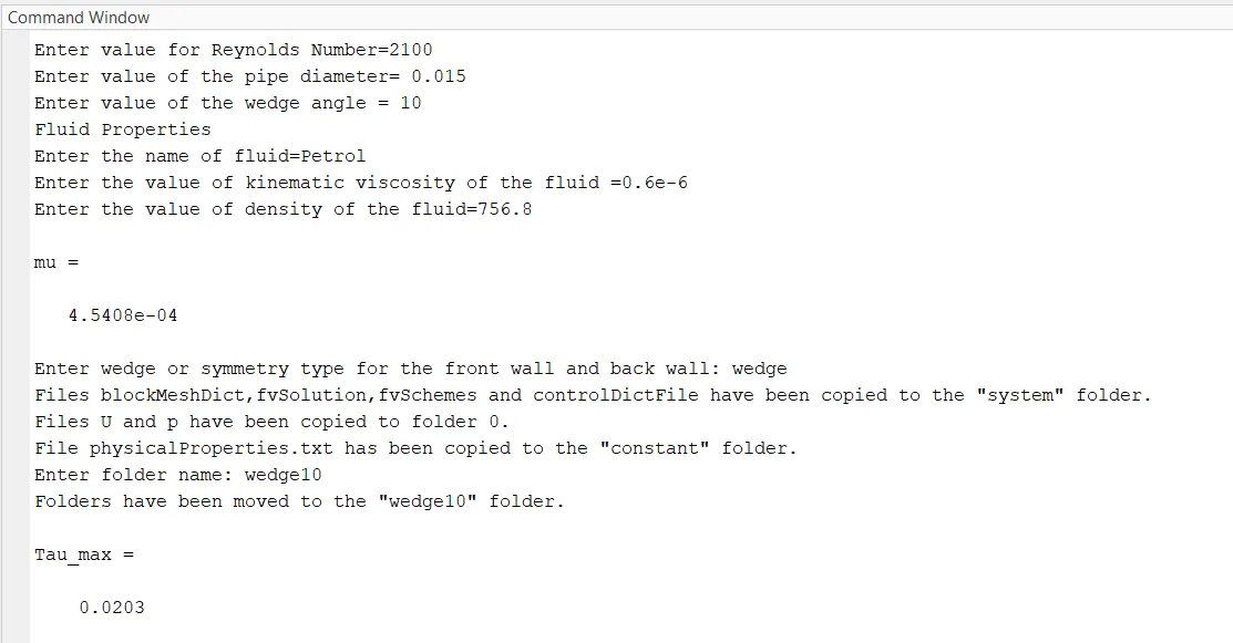
In summary, this MATLAB script is a comprehensive tool for setting up and running a simulation of fluid flow in a pipe using OpenFOAM, complete with user input, parameter calculations, file generation, and analytical validation.Executing the program to create different files for wedge and symmetry boundary condition that can be used in openfoam.
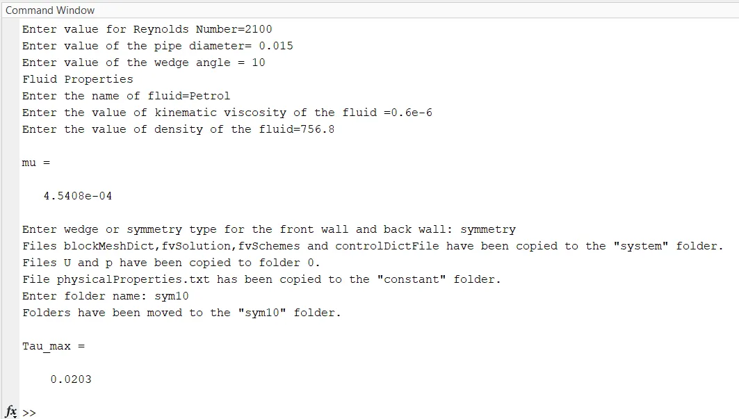
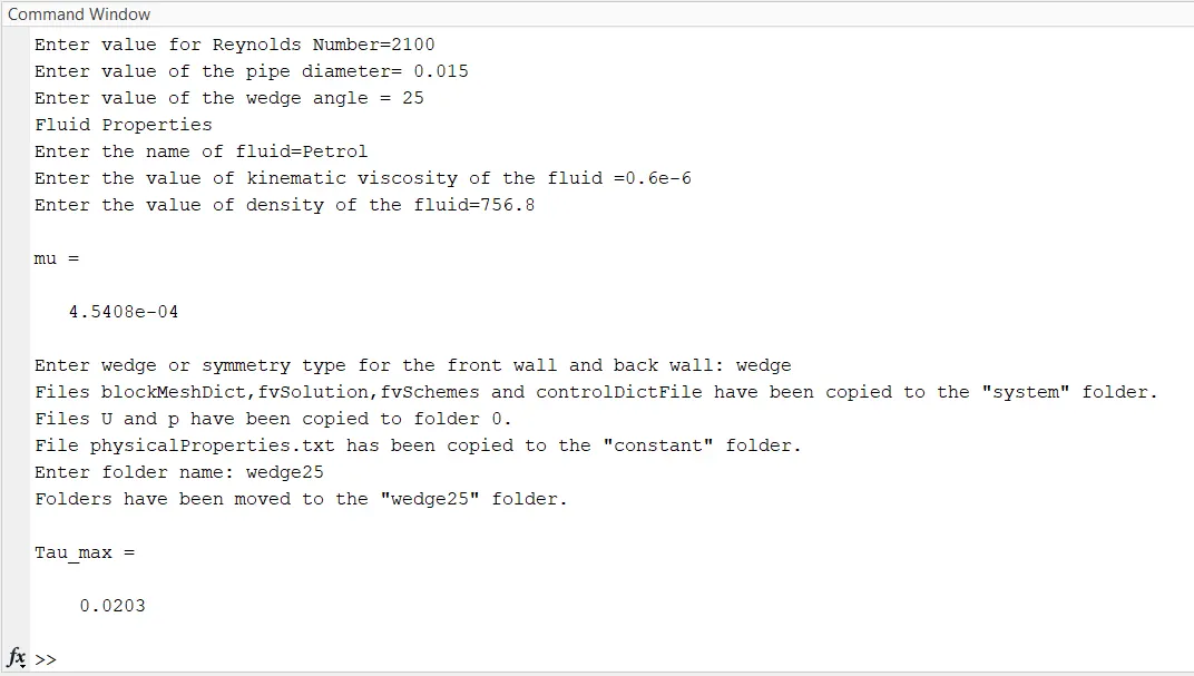
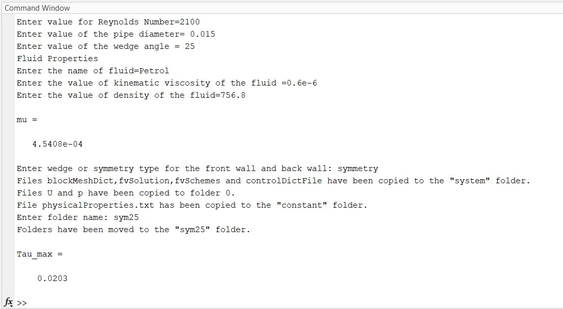
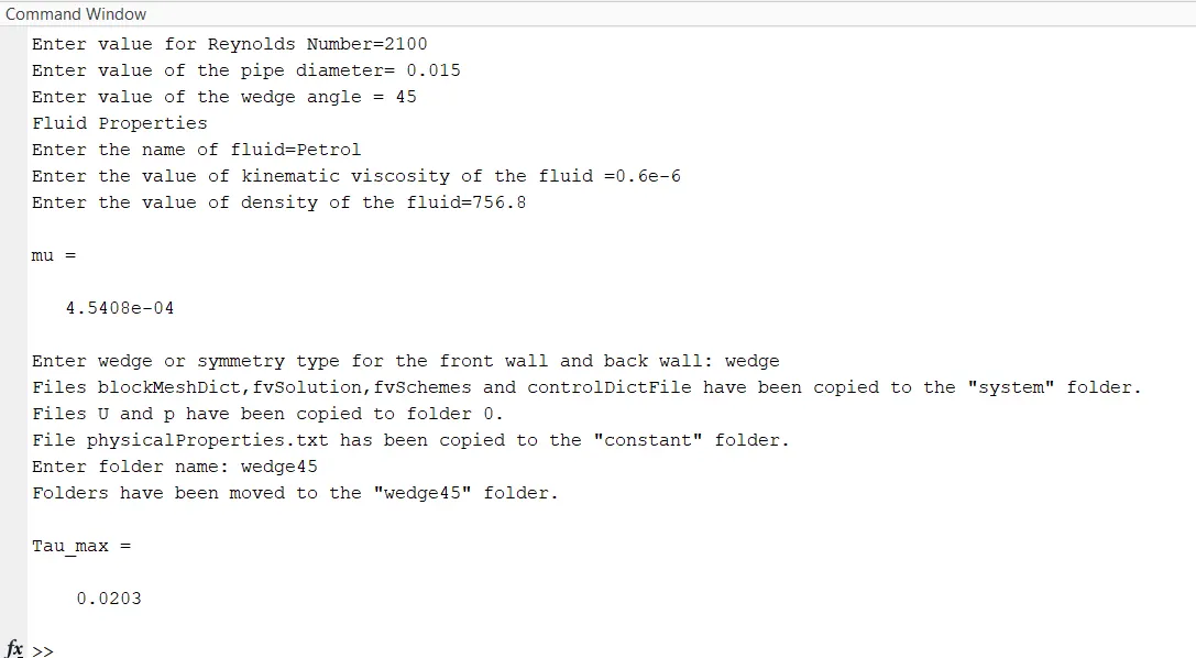
For different wedge angles creating openfoam files:
(i) wedge angle =10
BC: wedge
BC:symmetry
(ii) wedge angle=25
BC: wedge
BC: symmetry
(iii) wedge angle=45
BC: wedge
BC:symmetry
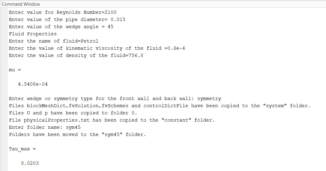
ANALYTICAL PRESSURE:
Using Haigen poisuelle flow equations
Analytical pressure:
Using Haigen poisuelle flow equations
Avg velocity, V_avg=`(Re*mu)/(rho*d)`=0.084 m/s
Maximum velocity, Vmax=2*V_avg =0.168 m/s
Piezo metric pressure drop, `gradp=(32*mu*V_(avg)*0.1*Lhydro)/d^2`
Kinematic pressure, Kinematic_p=`grad p`/rho=0.0011 Pa
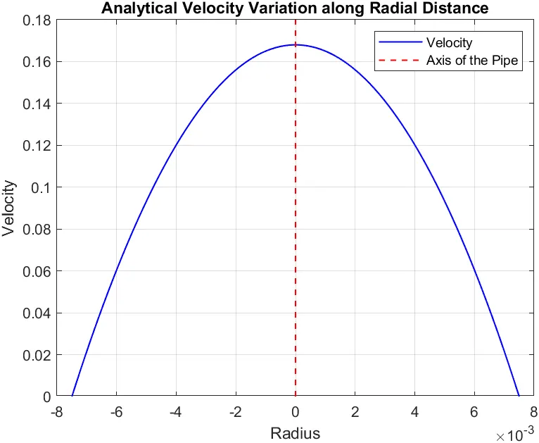
Files created are copied to the Openfoam main folder $FOAM_RUN.
In the linux system, use terminal to simulate with the help of openfoam.
steps to run simulation in Openfoam:
- open $FOAM_RUN folder by using cd $OPEN_RUN command.
- Access the required folder by using cd (name of the folder).
- Then mesh the geometry using blockMesh command.
- Use icofoam solver using icoFoam command.
- Then post processing is to be done in the paraview, use paraFoam command.
- Use reflect tool along y axis and plotline tool to make plots for velocity and pressure at fully developed region.
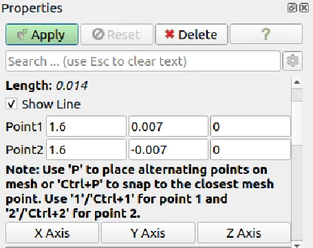
- To Calculate shear stress and plot the shear stress along the diameter of pipe:
- Enable the Common toolbar under View -> Toolbars -> Common.
- Click on the Calculator tool in the extreme left of the Common toolbar.
- In the Calculator, compute the magnitude of vector field U by typing mag(U) inside the calculation box and name the result array (e.g., mag_U).
- Click Apply to compute and apply the magnitude of velocity vector U in the Field Variable selection box.
- Press ‘Ctrl+Space’ or Click on Filters -> Search, search for 'Gradients of unstructured data set,' and click on it.
- In the Properties window, select the array name (e.g., mag_U) as the Scalar Array.
- Type a desired Result Array Name (e.g., grad_mag_U) for storing gradients of U_magnitude values.
- Click Apply to create a new quantity with the specified name inside the Field Variable selection box.
RESULTS:
For different wedge angles:
(i) wedge angle =10
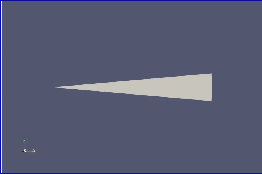
Velocity profile after using reflect tool along y-axis:
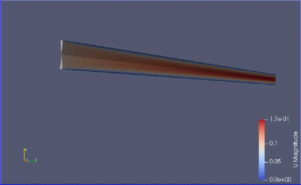
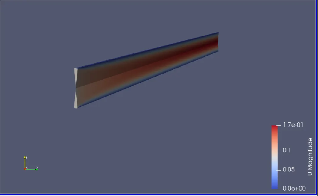
(a) wedge B.C. (b)Symmetry B.C.
Pressure profile after using reflect tool along y-axis:
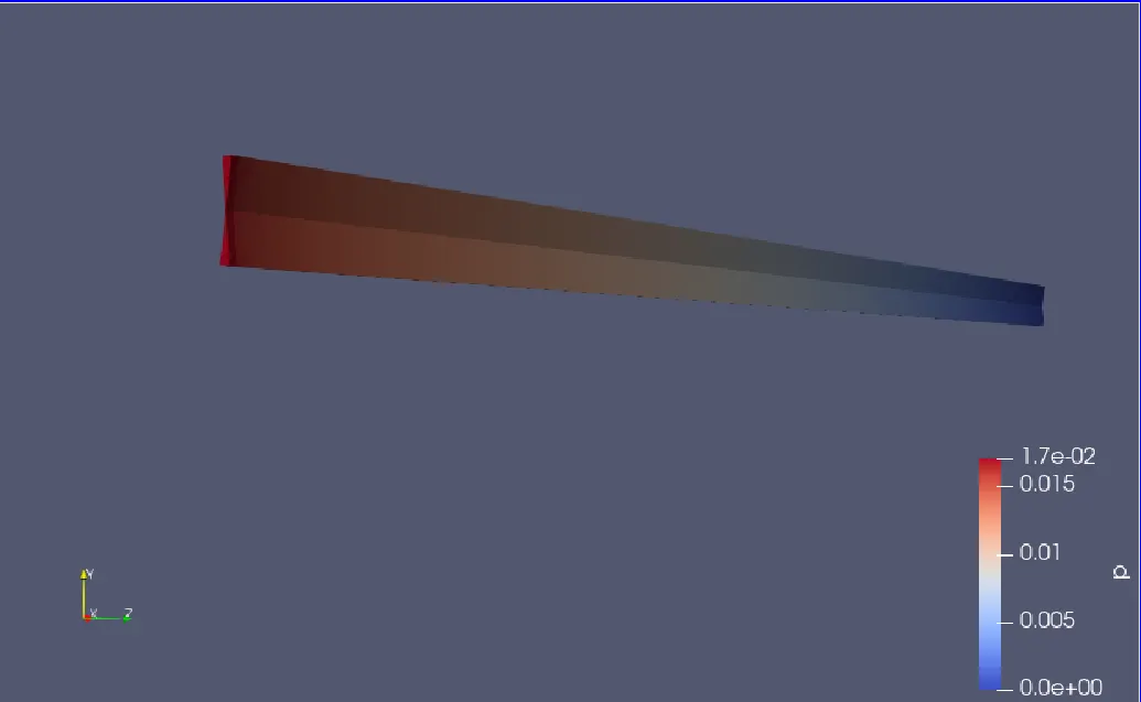
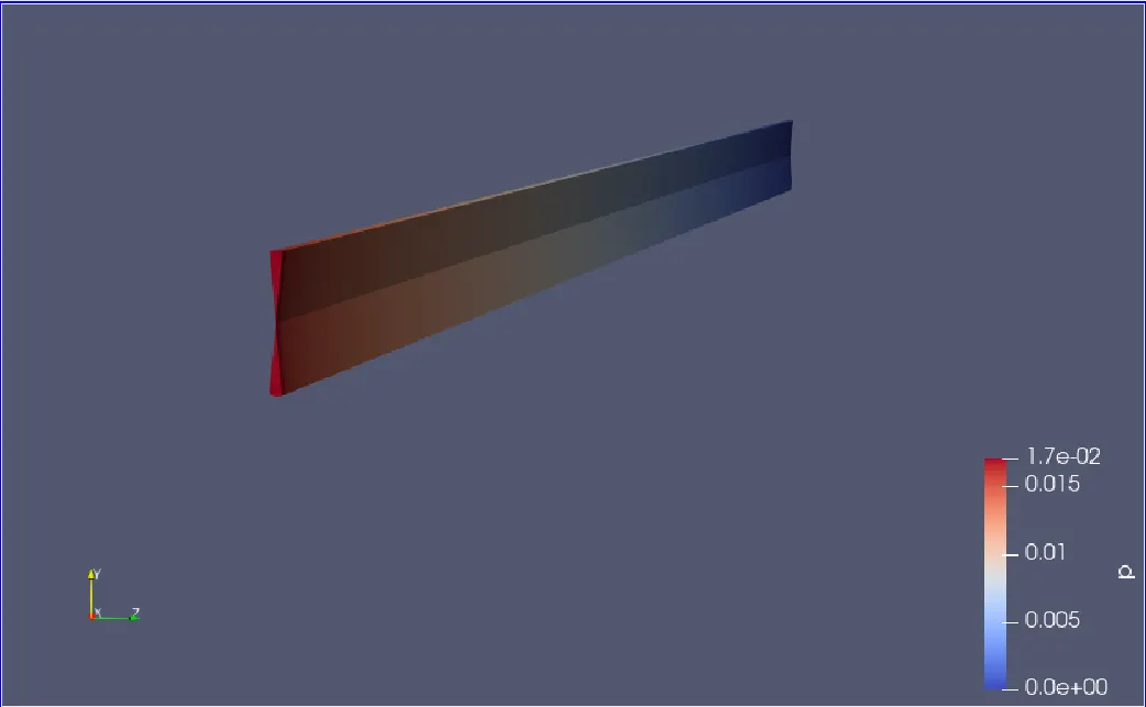
(a) wedge B.C. (b)Symmetry B.C.
BC: wedge BC:symmetry
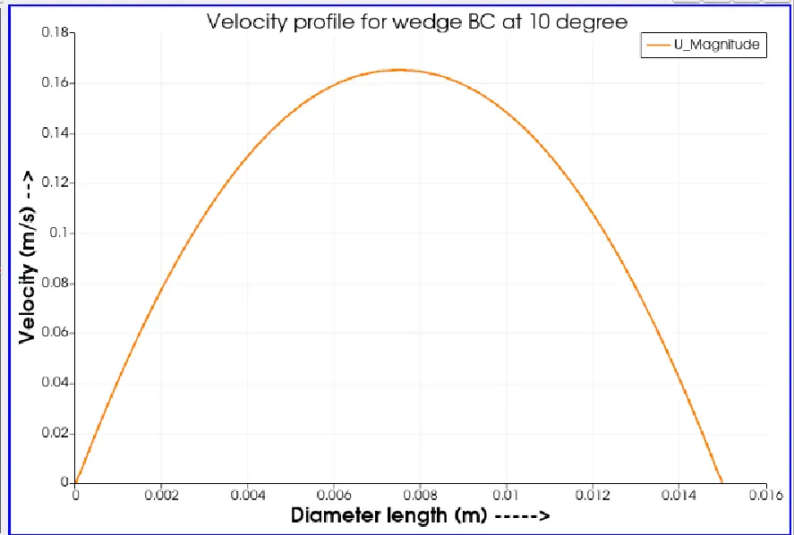
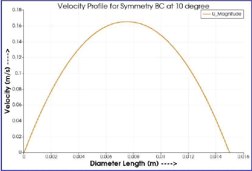
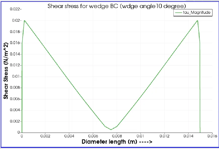
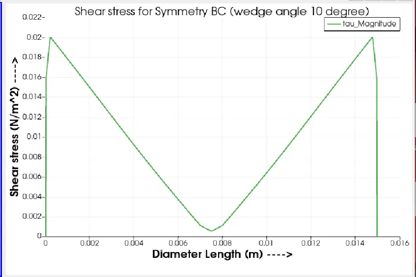
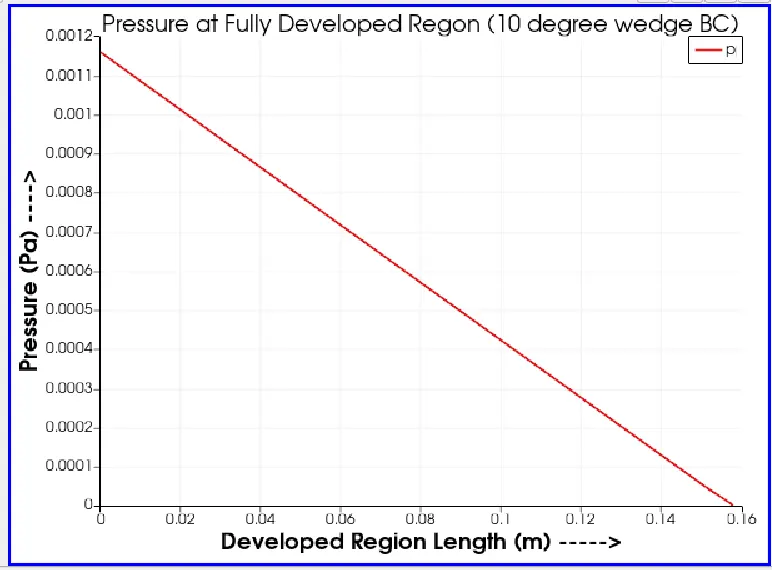
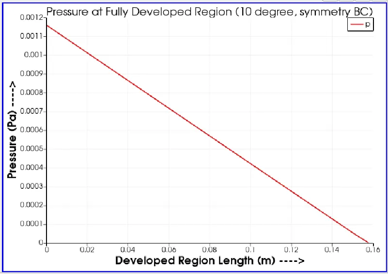
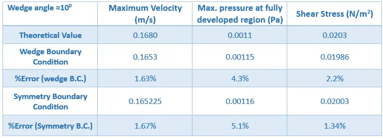
Here, we can see that the error in velocity of wedge and symmetry B.C. are nearly same. The error in pressure value is more in case of symmetry B.C. but the shear stress of the symmetry B.C. is very low.
(ii) wedge angle=25
Velocity profile after using reflect tool along y-axis:
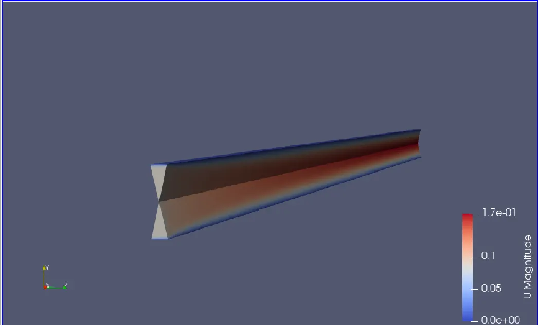
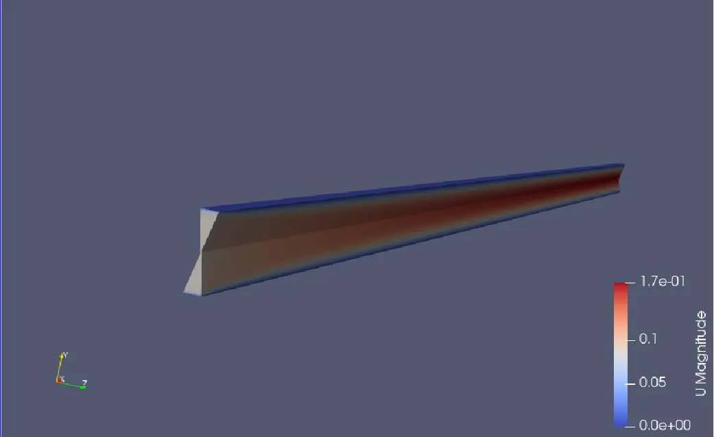
(a) wedge B.C. (b)Symmetry B.C.
Pressure profile after using reflect tool along y-axis:
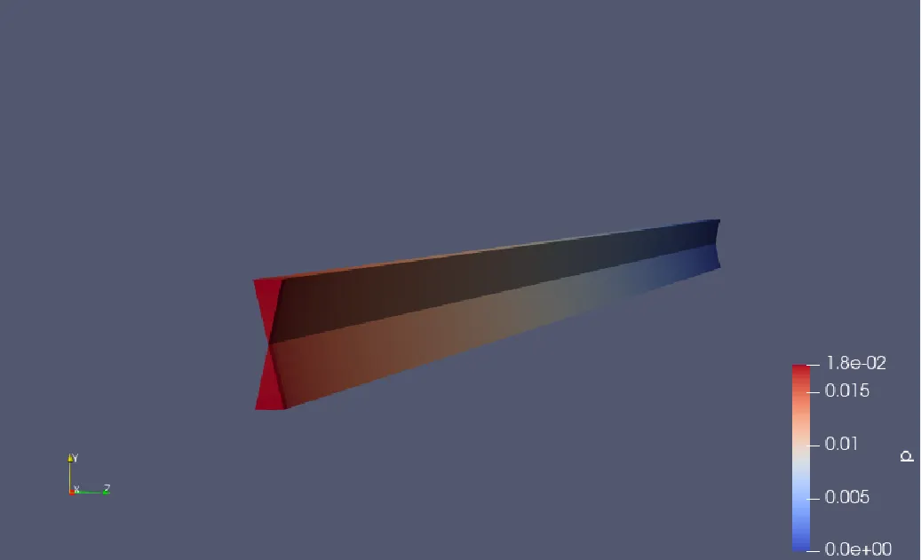
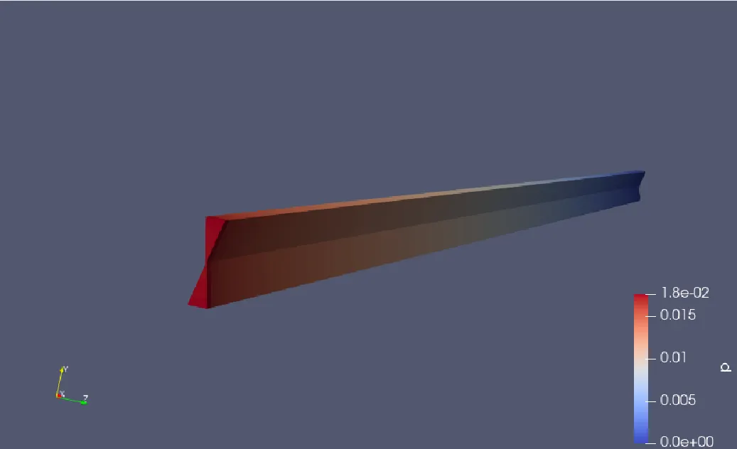
(a) wedge B.C. (b)Symmetry B.C.
BC: wedge BC:symmetry
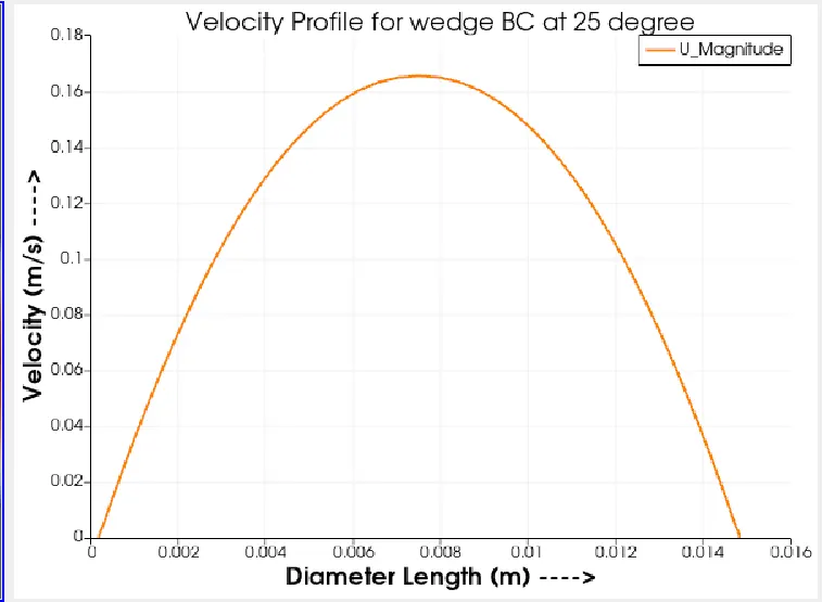
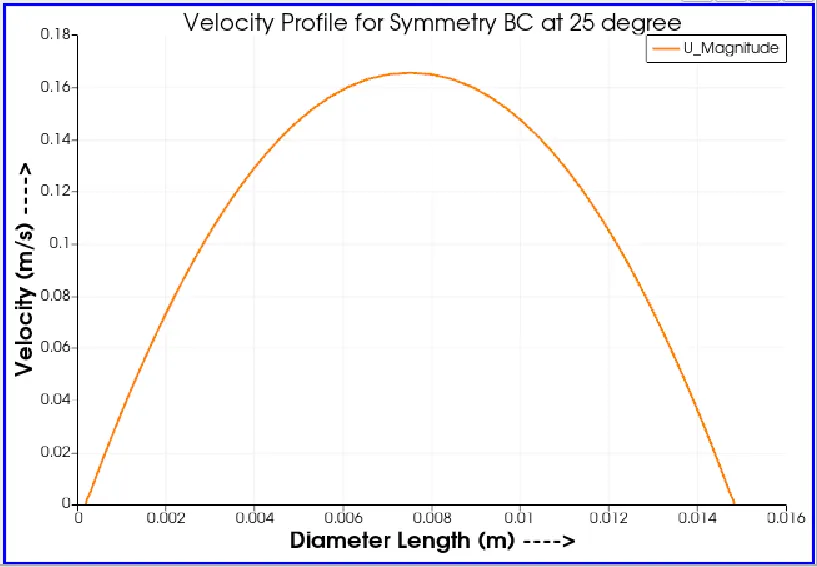
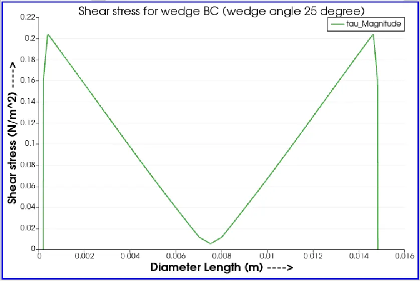
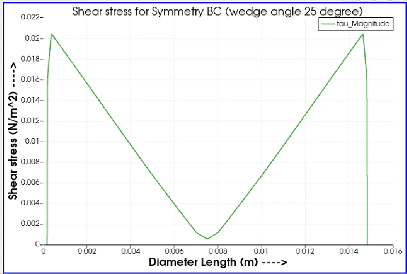
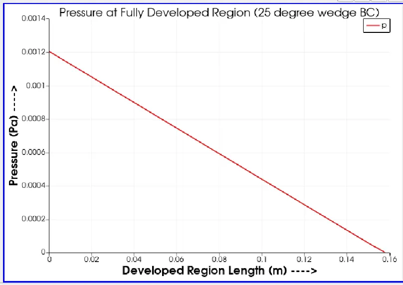
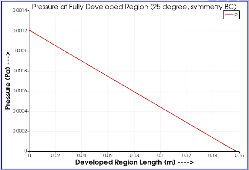
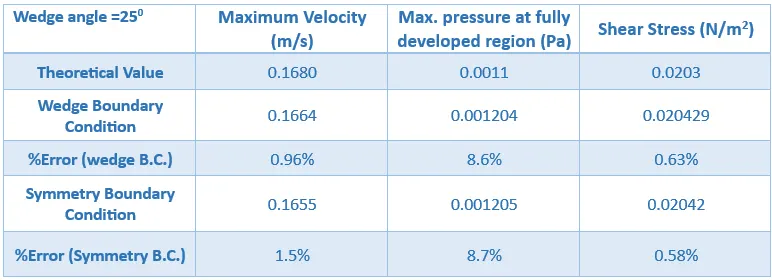
The error in velocity of wedge is very less than the symmetry B.C. The error in pressure value is more in case of symmetry B.C. but the shear stress of the symmetry B.C. is very low.
(iii) wedge angle=45
Velocity profile after using reflect tool along y-axis:
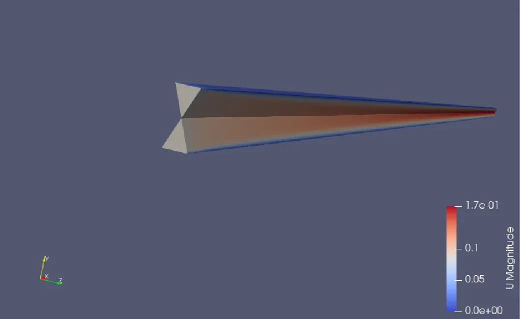
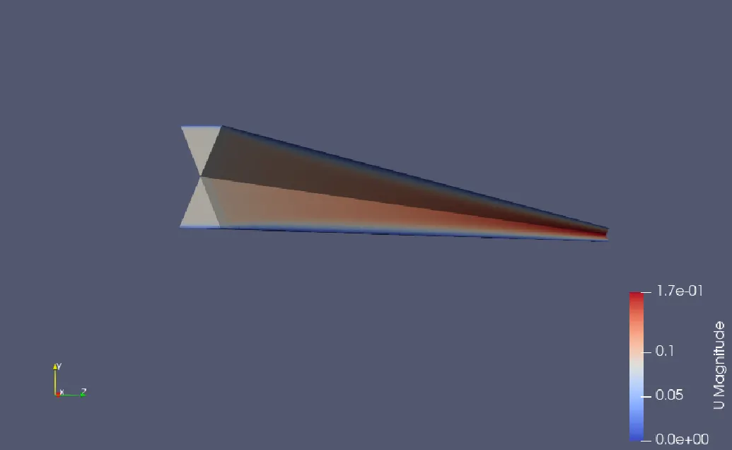
(a) wedge B.C. (b)Symmetry B.C.
Pressure profile after using reflect tool along y-axis:
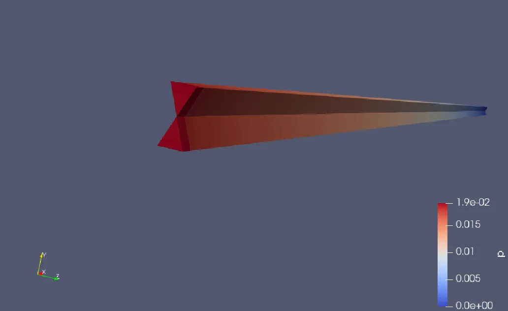
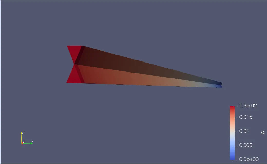
(a) wedge B.C. (b)Symmetry B.C.
BC: wedge BC:symmetry
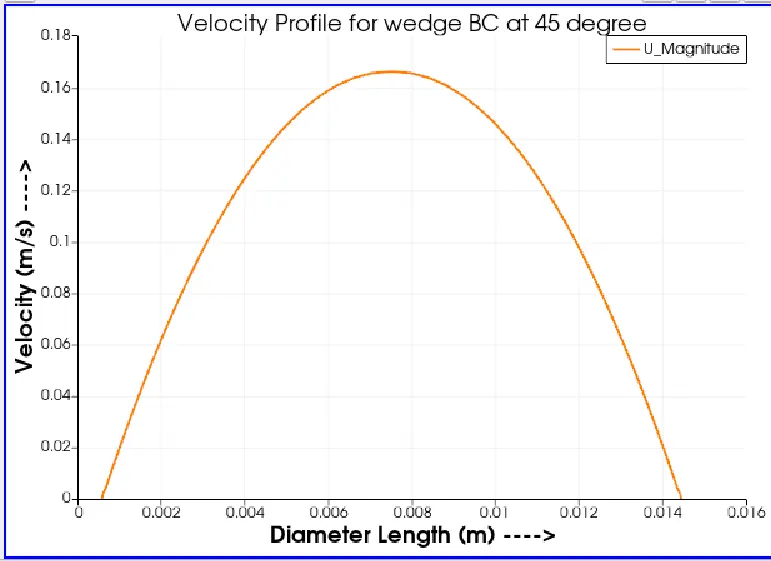
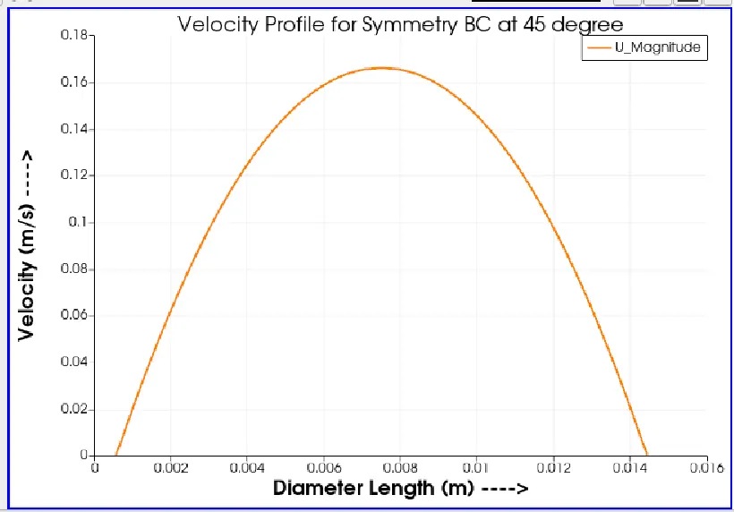
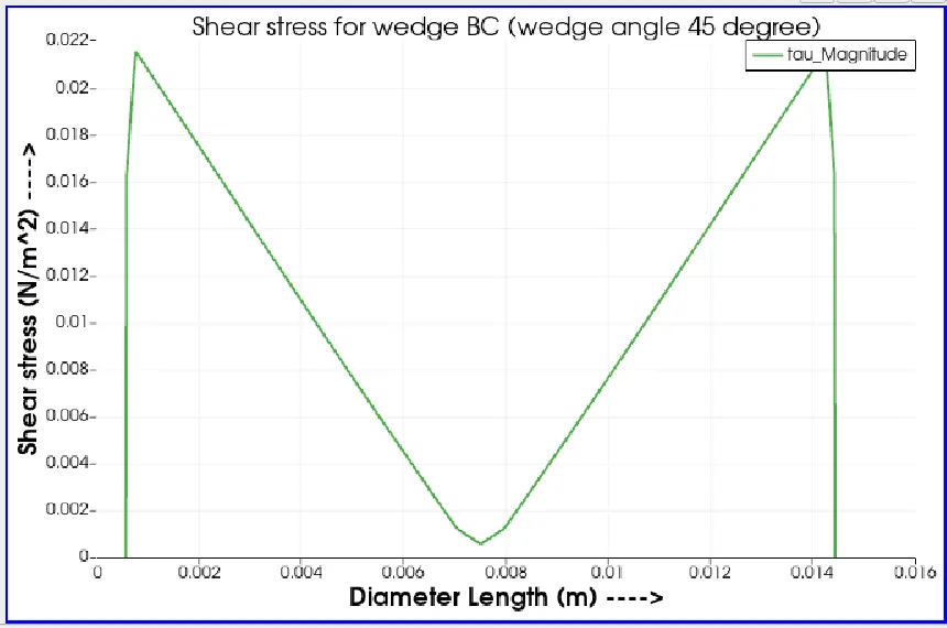
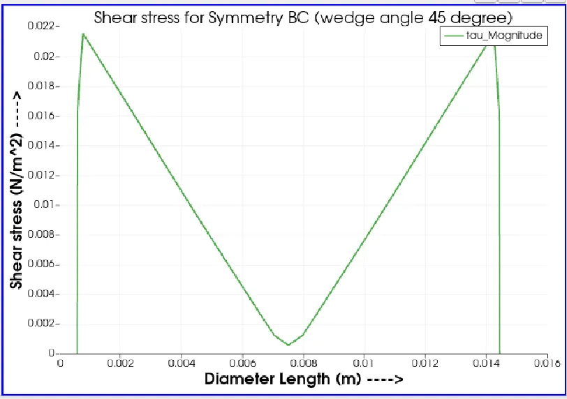
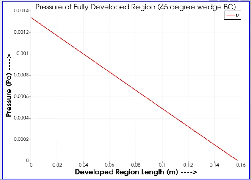
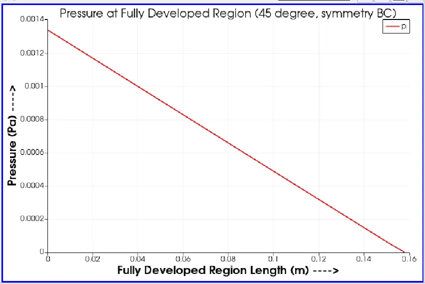
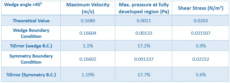
From the above table: the error in velocity of wedge and symmetry B.C. are nearly same. The error in pressure value is more in case of symmetry B.C. but the shear stress of the symmetry B.C. is very low.
As per the graphs and data obtained, it can be concluded that:
- Symmetry boundary conditions yield improved outcomes for shear stress but introduce slightly more error in estimating maximum velocity and pressure at the fully developed region compared to theoretical values. However, this discrepancy is relatively minor when contrasted with the effects observed with wedge boundary conditions.
- As the angle values increased from 10 degrees to 45 degrees, a marginal but consistent decrease in velocity error was observed. However, in the case of pressure and shear stress, the error exhibited an increasing trend.
CONCLUSION:
- Symmetry Boundary Condition, while showing minimal change in maximum velocities, contributes to slightly higher execution times compared to Wedge Boundary Condition.
- The Courant number experiences a slight increase with growing wedge angles, highlighting the significance of Symmetry Boundary Condition for result accuracy.
- Symmetry Boundary Condition, treating the mesh as three-dimensional, allows calculations along all three global axes, enhancing accuracy.
- Despite trade-offs in simulation times, the fundamental physics of the problem remains consistent, ensuring reliable results.
- Symmetry Boundary Condition yields superior outcomes for shear stress but introduces a slightly higher error in estimating maximum velocity and pressure.
- The fluctuations in wedge angles impact the velocity error, showing a decrease, while the errors in pressure and shear stress exhibit an increase. This underscores the subtle and intricate interplay of boundary conditions and geometry on the outcomes of the simulation.