Week 5 - Rayleigh Taylor Instability

AIM:

Conducting a Rayleigh Taylor Computational Fluid Dynamics (CFD) simulation.

OBJECTIVES:

• Delve into various CFD models employed to address Rayleigh Taylor Instability problems, elucidating their theoretical underpinnings and practical applications.
• Conduct a Rayleigh Taylor instability analysis utilizing the Volume of Fluid (VOF) multiphase model. The simulation involves two distinct mesh element sizes: Mesh size - 0.5mm, incorporating water and air and Mesh size - 0.1mm, featuring water and air.
• Extend the simulation to include water and a user-defined material characterized by density = 400 kg/m³ and viscosity = 0.001 kg/m-s. Conduct a comparative analysis of their behaviors under the same mesh size (0.1mm).
• Define and derive the Atwood number for each case, offering insights into the degree of instability present in the simulations.
• Elaborate on the effect of the Atwood number on instability, providing a comprehensive understanding of how variations influence the observed behaviors.

This structured approach aims to not only perform simulations but also to provide a comprehensive understanding of the underlying models, behaviors, and the influence of parameters such as mesh size and Atwood number on the Rayleigh Taylor instability

INTRODUCTION:

The Rayleigh–Taylor instability, often referred to as RT instability, represents an intriguing phenomenon occurring at the interface between two fluids characterized by different densities. This instability arises when the lighter fluid exerts a force, pushing against the heavier fluid. Instances of this behavior are observed in various natural occurrences, such as the suspension of water above oil under the influence of Earth's gravity, the formation of mushroom clouds resulting from volcanic eruptions and atmospheric nuclear explosions, and the explosive events in supernovae where expanding core gas is accelerated into denser shell gas. RT instability is also a factor in the instabilities witnessed in plasma fusion reactors and inertial confinement fusion processes.

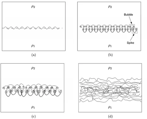
This illustration depicts the progression of Rayleigh–Taylor instability, starting with small wavelength perturbations at the interface (a), evolving into distinctive mushroom-shaped spikes and bubbles (fluid structures of heavy into light fluid) (b). The interaction of these fluid structures occurs through processes like bubble merging and competition (c), ultimately leading to the formation of a mixing region (d). In the figure, ρ2 represents the heavy fluid, ρ1 represents the light fluid, and gravity acts downward, rendering the system Rayleigh–Taylor unstable.

As RT instability progresses, the initial perturbations undergo a transition from a linear growth phase to a non-linear growth phase, eventually giving rise to distinctive fluid structures known as "plumes" ascending and "spikes" descending. In the linear phase, fluid movements can be approximated closely using linear equations, and the amplitude of perturbations undergoes exponential growth over time. Contrastingly, in the non-linear phase, the perturbation amplitude becomes too substantial for linear approximations, necessitating the use of non-linear equations to describe fluid motions. The structure of subsequent non-linear RT instability flows is predominantly determined by the density disparity between the two fluids. This structural determination is contingent upon the Atwood number (A), defined as the difference in fluid densities divided by their sum. For Atwood numbers close to 0, RT instability flows exhibit symmetric "fingers" of fluid, while for Atwood numbers close to 1, the much lighter fluid beneath the heavier fluid takes the form of larger bubble-like plumes.

The ubiquity of the RT instability process extends beyond terrestrial examples, encompassing phenomena in astrophysics and electrohydrodynamics. For instance, the Crab Nebula illustrates the presence of RT instability structure, where the expanding pulsar wind nebula, fueled by the Crab pulsar, sweeps up ejected material from a supernova explosion that occurred a millennium ago. Recently, RT instability has been discerned in the Sun's outer atmosphere, specifically the solar corona, where a relatively dense solar prominence overlays a less dense plasma bubble. This case bears a resemblance to magnetically modulated RT instabilities.

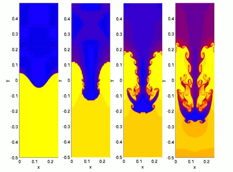
The evolutionary trajectory of RT instability unfolds in four key stages. In the initial stage, perturbation amplitudes, in comparison to their wavelengths, are small, allowing linearization of the equations of motion and resulting in exponential instability growth. The formation of mushroom-shaped spikes and bubbles becomes evident as non-linear effects emerge towards the conclusion of this stage. The second stage witnesses the continued growth of mushroom structures, modeled using buoyancy drag models, with a growth rate approximately constant in time. Nonlinear terms in the equations of motion become crucial at this juncture. The third stage is marked by interactions between spikes and bubbles, encompassing bubble merging and competition. Bubble merging involves the combination of smaller spikes and bubbles into larger ones through nonlinear mode coupling. Simultaneously, bubble competition sees saturated spikes and bubbles of smaller wavelength enveloped by larger ones that are yet to saturate. The culmination of these interactions results in the fourth and final stage – a region of turbulent mixing. It is generally assumed that the developed mixing region is self-similar and turbulent, provided that the Reynolds number attains a sufficiently large value.

The practical CFD Models that have been based on the mathematical analysis of Rayleigh Taylor Waves are as follows :

1. Richtmyer-Meshkov Instability:The Richtmyer-Meshkov instability manifests at the interface between two fluids when impulsively accelerated, often by a shock wave. It leads to hydrodynamic instability, nonlinear growth, and a subsequent transition to turbulence.
   
   Example: In practical terms, consider the supersonic combustion occurring in scramjets. The Richtmyer-Meshkov instability plays a crucial role during combustion processes, supernova explosions, and in hypersonic air-breathing engines.
   
   
2. Turbulence Model: Turbulence models are vital for predicting average mixing behavior in flows that are typically one- or two-dimensional. These models simplify the complex equations governing turbulent flows to predict their statistical evolution.
   
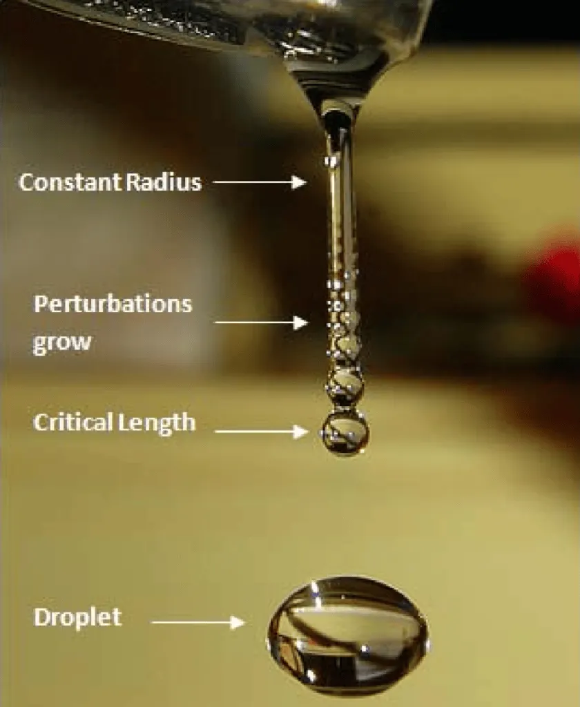
   Example: In the context of CFD simulations, turbulence models are employed to understand and predict the evolution of turbulence. For instance, in simulating airflow over an aircraft wing, turbulence models help analyze the mixing and flow patterns.
   
   
3. Plateau–Rayleigh Instability: Also known as Rayleigh instability, this model explains the phenomenon where a falling stream of fluid breaks into smaller packets with reduced surface area. The driving force is the tendency of liquids, due to surface tension, to minimize their surface area.
   
   Example: Inkjet printers utilize the Plateau–Rayleigh instability. A jet of liquid is perturbed into a steady stream of droplets, forming the basis for the controlled release of ink droplets onto paper.
   
   
4. Kelvin–Helmholtz Instability: Observed in scenarios of velocity shear within a single continuous fluid or at the interface between two fluids with a velocity difference. This instability is responsible for the formation of basic structures in nature.
   
   Example: In meteorology, the Kelvin–Helmholtz instability is evident in cloud formations and ocean waves. It is also responsible for the appearance of Saturn's bands and the sun's corona.
   
   
5. Smoothed Particle Hydrodynamics (SPH) Method:SPH is a computational method used for simulating the mechanics of continuum media. It ensures mass conservation and creates a free surface for interactions between fluids by representing denser fluid as particles and empty space as lighter fluid.
   
   Example: SPH finds application in simulating fluid flows in various industries, such as aerospace and automotive. It excels in scenarios where traditional grid-based techniques may struggle to capture complex fluid dynamics.
   
   
6. Single Fluid Model:The single fluid model is applied in the analysis of two-phase flows, treating individual fluid phases as a flowing mixture. It consists of five equations describing mass, momentum, and energy for a vapor/liquid mixture, along with equations for the formation and growth of the liquid phase.
   
   Example: In nuclear reactor simulations, the single fluid model is used to understand the behavior of the coolant as it interacts with the reactor core.
   
   
7. Two Fluid Model:This model separates governing equations for vapor and liquid phases but doesn't account for interactions between droplets, heat exchange, and the velocity slip between vapor and liquid phases.
   
   Example: In studying the behavior of fuel and oxidizer in combustion processes, the two fluid model helps analyze the dynamics of each phase independently.
   
   
8. Discrete Boltzmann Model:Deployed for premixed, non-premixed, or partially premixed non-equilibrium reactive flows, this model is designed to investigate hydrodynamic and thermodynamic non-equilibrium effects in phase separation processes.
   
   Example: In the context of combustion studies, the Discrete Boltzmann Model aids in understanding the intricate interactions and deviations from thermodynamic equilibrium in reacting flows, providing insights into combustion efficiency and stability.

Mathematical Models that have been adapted for CFD calculations are as follows:

• Mass Diffusion Model:This model meticulously accounts for the diffusion of mass within a fluid, emphasizing the distribution and movement of different substances over time. It incorporates principles of concentration gradients and molecular diffusion, making it invaluable in scenarios involving chemical reactions, species transport, and intricate diffusion processes, such as in environmental studies and industrial chemical processes.
  
  
• Single Fluid Model: In the Single Fluid Model, the assumption is made that distinct fluid phases behave collectively as a single, continuous mixture. This simplification is especially useful in the simulation of two-phase flows, where multiple fluids coexist but are treated as a unified entity. This model finds applications in diverse fields ranging from hydraulic systems to thermal management studies.
  
  (a) Potential Flow Model:The Potential Flow Model simplifies fluid dynamics by assuming incompressibility and irrotationality, neglecting viscosity effects. Widely employed in aerodynamics and scenarios where viscous forces are negligible, this model streamlines calculations by focusing on the fundamental potential energy of the fluid, providing insights into lift, drag, and flow patterns around objects.
  
  (b) Buoyancy Drag Model:The Buoyancy Drag Model integrates the impact of buoyancy forces and drag forces on fluid flow, particularly addressing situations with varying fluid densities. It plays a crucial role in natural convection studies, where buoyancy-driven flows significantly influence heat and mass transfer, making it applicable in environmental modeling and heat exchanger design.
  
  (c) Besnard-Harlow-Rauenzahn (BHR) Model:Tailored for simulating two-phase flows, the BHR Model considers interactions between dispersed and continuous phases. It accounts for the dynamics of mixtures, such as liquid droplets in a gas, offering a detailed representation of phase interactions. Applications include combustion studies, liquid spray simulations, and nuclear reactor analyses.
  
  
• Multi-Fluid Model:The Multi-Fluid Model goes beyond the Single Fluid Model by treating different fluid phases independently, each governed by its unique set of equations. This approach is advantageous when distinct phases demand individualized attention, like simulating air-water interfaces in maritime engineering or studying multiphase flows in oil and gas pipelines.
  
  Two, Three, and Four-Equation K-L Turbulence Models: These turbulence models quantify the transport of turbulent kinetic energy (K) and its dissipation rate (L), offering a comprehensive framework for simulating turbulent flows of varying complexities. They are extensively used in industries where turbulence plays a crucial role, such as aviation, automotive design, and environmental fluid dynamics.

GEOMETRY SETUP:

• Begin by selecting Fluent in the Workbench setup, then proceed to edit the geometry using SpaceClaim.
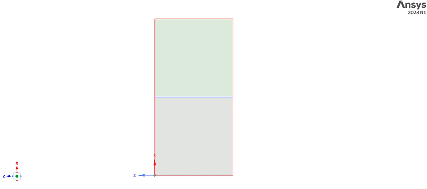
• In SpaceClaim, choose the XY plane to sketch a 2D geometry. Create a square with dimensions of 20mm using the sketch tool. Utilize the pull tool to convert the sketch into a surface.

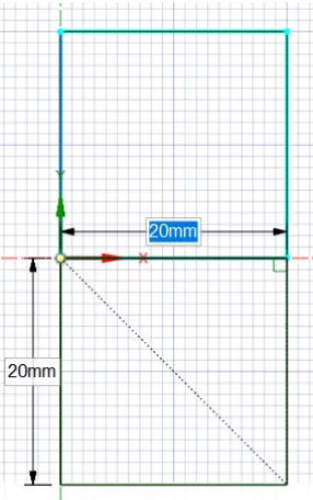
• Transfer the created geometry to a new component and assign the name "fluid 1" to this component.
• Generate a new geometry within the main design and designate it as "fluid 2." Create a square of 20mm directly above the previously defined Air square, establishing an interface between the two geometric entities.
• Perform a share preparation by selecting the entire geometry under the Workbench. Utilize the share option to enable the exchange of information between the two phases. This ensures conformal meshing can be achieved across the interface, promoting accurate simulation results.
  

Procedure:

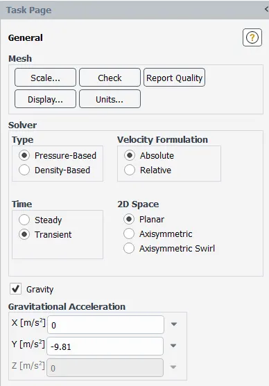
1. Choose the pressure-based solver and opt for the transient state approach.
2. Specify gravity with X = 0 m/s² and Y = -9.81 m/s².
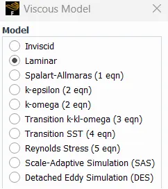
3. Select the viscous model and opt for the Laminar model.
4. In the multiphase model, choose the Volume of Fluid model and set the implicit formulation.
5. Omit the Energy equation, as temperature is not a factor in this simulation.
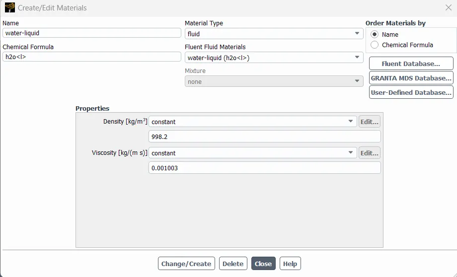
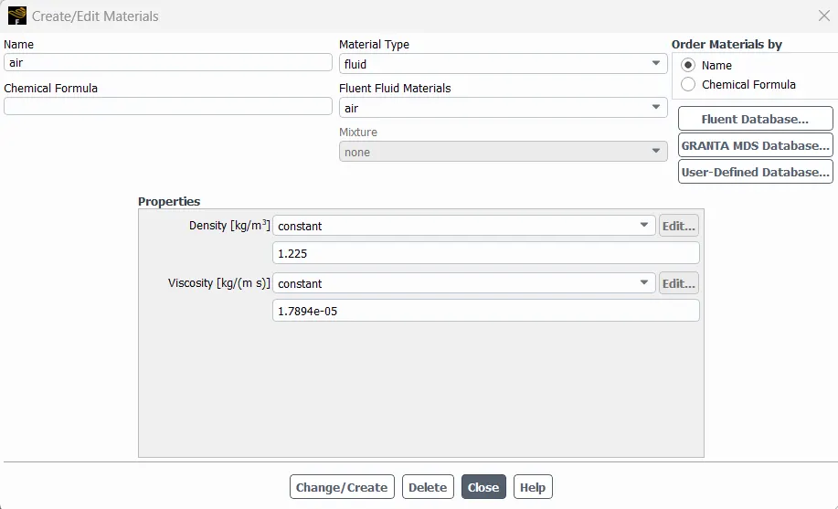
6. Add materials by selecting 'air' and 'water' from the Fluent Database Materials for case1 and case . For case 3 add water and user defined fluid.
7. Navigate to multiphase, click on phases, designate 'air' as the primary phase material, and 'water' as the secondary phase material for first two cases. Designate 'User defined fluid' as the primary phase material, and 'water' as the secondary phase material for case3.
8. Verify that the bottom surface is 'air' and the upper surface is 'water' in the domain.
9. Perform a mesh check to ensure its validity.
10. Initialize the problem using the standard initialization method, as a transient state approach is employed.
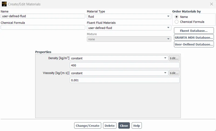
11. In the third simulation case, replace 'air' with a user-defined material in Materials and set it as the Primary phase, keeping 'water' as the second phase material.
12. Review the domain, inspect the zones, and visually identify surfaces for patching.
13. Use the standard initialization method and click "t=0 Initialize."
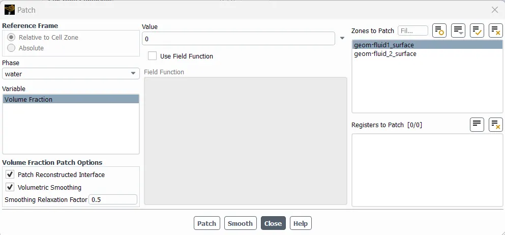
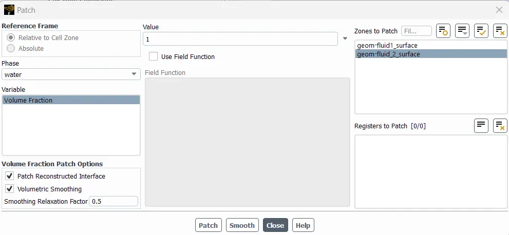
14. Navigate to Patch, set the Volume fraction to 1 for the water surface and 0 for the air surface.
15. Under solutions - calculation activities, double click on Run-calculation, choose the Fixed type, set the number of time steps, and the timestep size.
16. Create a Contour for Volume Fraction for the water phase.
17. Generate a Time step animation for the Volume fraction of water every two time steps.
18. Run the calculation and wait for completion. If encountering floating-point errors, recheck the mesh quality, aspect ratio, and element size. Ensure proper meshing and re-run the calculation, remembering to patch the volume fraction of water to 1 whenever re-running.

CASES:

Case 1:

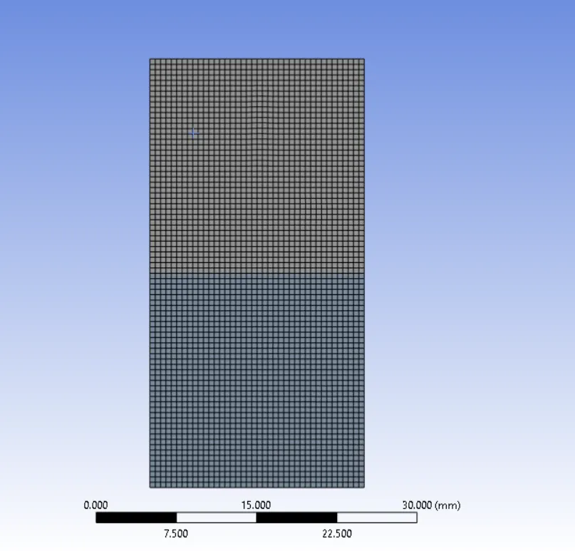
Mesh size - 0.5 mm

Materials: Water and air

FLUENT SETUP:

Genral setup:

Viscous Model:

Fluid Materials:

Phases: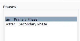

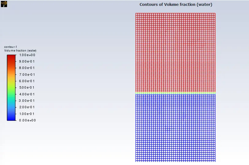
Fluid1 is the bottom and fluid2 is the uper portion of the 2D model, patching:

Volume of water(red):volume of air(blue) :

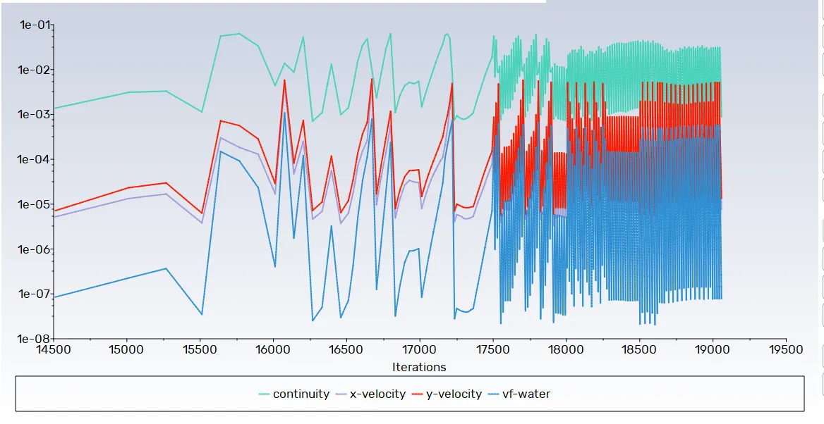
Residual Plot:

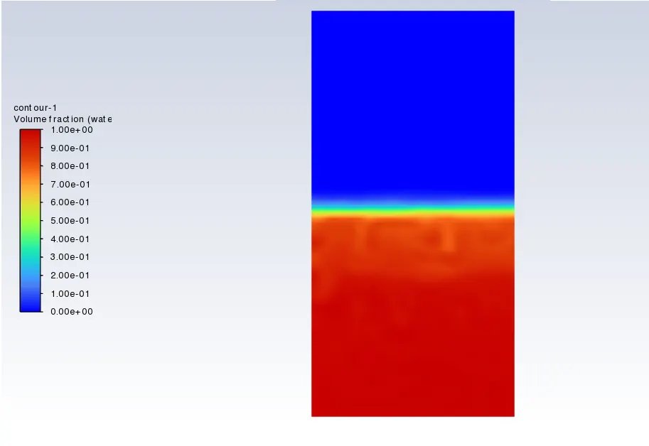
Final Contour:

Case 2:

Mesh size - 0.1mm

Materials: Water and air

Finer mesh:

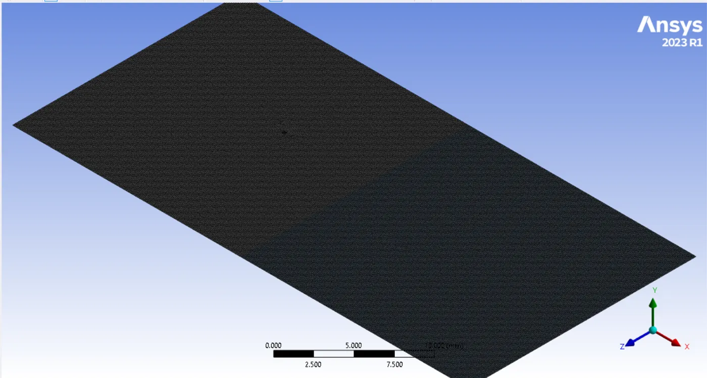
Use same fluent setting and use proper time-step and time-step size.

Upper Portion represents Water(α=1)

Lower Portion Represents Air ( α=0)

Initiazilation Method -> Hybrid

Solving Method -> coupled

Total Flow Time = (Time Step Size) * (No of Time Steps)

Residual Plot:

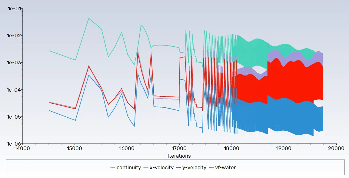
Final Contour:

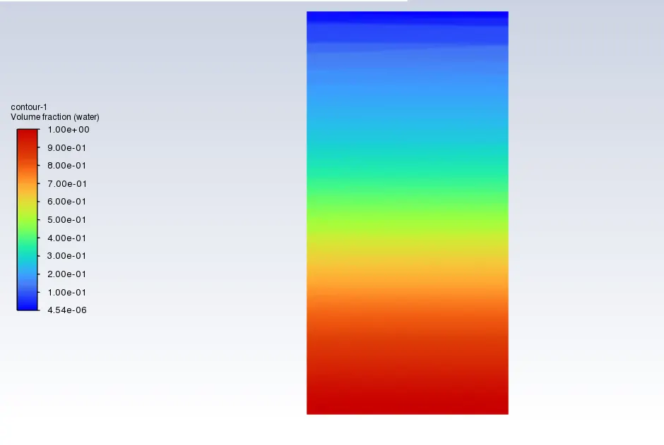
From observing case 1 and case 2:

In terms of computational considerations, a finer mesh better captures instability than a coarse mesh, although it requires more time for the heavier fluid to settle. While computationally expensive, the finer mesh produces more accurate results. Given the unpredictable nature of instabilities changing over time in the simulation, a transient approach is preferred over a steady-state approach.

Case 3:

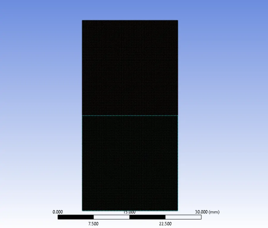
Mesh size - 0.1mm

Materials: Water and user-defined fluid (density = 400 kg/m³, viscosity = 0.001 kg/m-s)

Mesh:

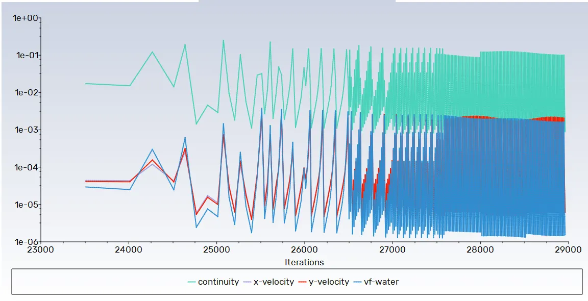
Residual Plot:

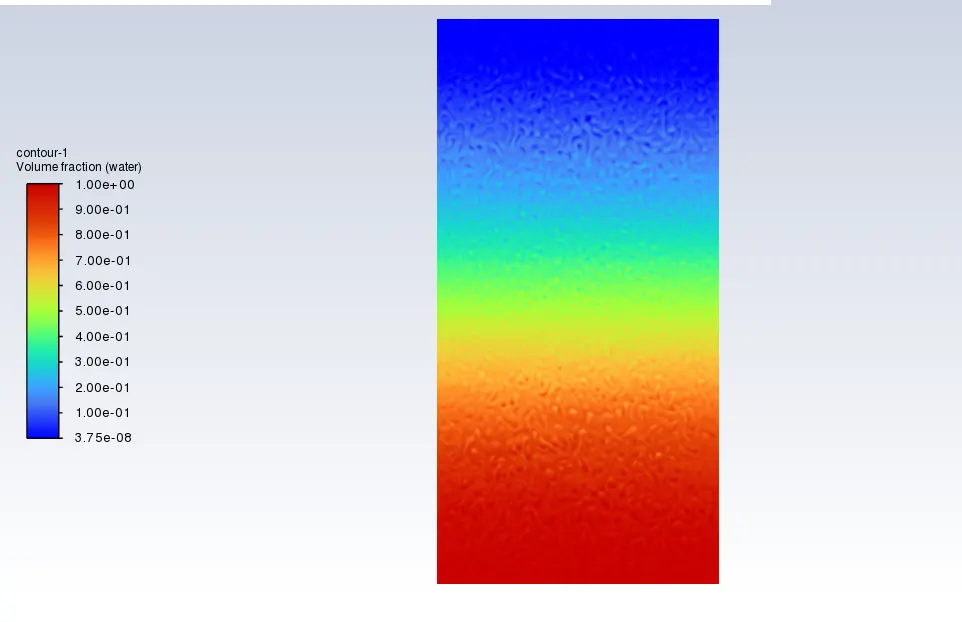
Final Contour:

A steady-state approach is unsuitable for simulations of phenomena like Rayleigh-Taylor Instability due to the following reasons:

• RTI involves dynamic, time-dependent processes, and a steady-state approach cannot capture the evolving nature of these phenomena.
• The transient nature of instabilities, shock waves, and fluid interactions in RTI requires a simulation approach that accounts for temporal changes.
• RTI exhibits unpredictable and turbulent behavior over time, which a steady-state simulation would overlook.
• The formation and evolution of shock waves in RTI are time-dependent, and a steady-state approach cannot represent the dynamic propagation of shock waves.
• RTI often involves turbulent mixing, and turbulence is inherently time-dependent, requiring a transient solver for accurate representation.
• RTI can be sensitive to initial conditions, and a steady-state approach may not consider the influence of initial transients on subsequent evolution.

Atwood Number:

In fluid dynamics, the Atwood Number is described as a dimensionless number that is used to explore hydrodynamic instabilities in density-stratified flows.

It is the ratio of difference in densities to the summation of the densities

`A = (ρ1 - ρ2)/(ρ1 + ρ2)`

where,

A = Atwood number,

`ρ1` = density of fluid 1

`ρ2` = density of fluid 2

Calculation Results Table

Mesh Type	Mesh Size	No of Elements	Materials Used	Atwood Number
BaseLine Mesh Simulation	0.5 mm	3200	Air and water-liquid	0.99754
Refined Mesh Simulation	0.1 mm	80000	Air and water-liquid	0.99754
Refined Mesh Simulation	0.1 mm	80000	user-defined-material and water-liquid	0.42784

The instability's behavior is influenced by the variation in Atwood number in the two mentioned (\\Air and water-liquid\\ & \\ user-defined-material and water-liquid \\) cases:

The Atwood number's influence on instability is evident in the three stages of Rayleigh Taylor Instability (RTI): Linear stability, Mushroom head falling or Bubble rise formation, and long-term evolution due to bubble merging and mixing.

In instances of low Atwood numbers (user-defined-material and water-liquid), the shapes of bubbles and mushroom heads are relatively symmetrical, with disturbances remaining linear for an extended period. Conversely, high Atwood numbers (Air and water-liquid) result in less symmetrical shapes that form rapidly, leading to a nonlinear growth rate.

• At Atwood Number close to zero, RTI forms symmetric fingers of fluid.
• At Atwood Number close to one, RTI results in lighter fluid forming larger bubble-like plumes.
• Instability sensitivity to time step and mesh size, requiring under-relaxation to prevent divergence.
• Mesh refinement clarifies instability patterns, revealing distinct volume fraction bands.
• Higher Atwood Numbers intensify instability, reducing settling time.

CONCLUSION:

• The simulation initiates in hydrostatic equilibrium, revealing Rayleigh Taylor instability at the interference of lower and higher density fluids, causing shock wave formation.
• Air bubble formation compresses the surrounding heavy fluid, generating multidimensional shock waves.
• Refining the mesh yields smoother simulation results at fluid interfaces. Finer mesh captures instability waves better but extends simulation time.
• Higher density fluid displacement leads to air bubble and vortex formation, traveling upward with time.
• Detailed results showcase wave formation and air bubbles initially trapped in the lower region, later traveling upward, generating shock waves.
• Despite phase separation, some diffusivity between air and water is observed. Sudden collapse in the layer between denser and lighter fluid causes time-dependent spike generation.
• User-defined material with higher density takes longer to settle compared to air.
• Simulation involves capturing time-dependent instabilities, making a transient approach preferable over steady-state. Steady-state is unsuitable as it is time-independent, whereas RTI requires studying time-dependent turbulent mixing.

Overall Conclusion:

• RTI simulation using VOF and transient solver provides valuable insights into time-dependent physics of turbulent mixing.
• Atwood Number variations impact instability characteristics, emphasizing the need for a transient approach in simulations.