Week 4 - CHT Analysis on Exhaust port
AIM:
The primary focus of the objectives lies in conducting a steady-state Conjugate Heat Transfer (CHT) analysis on the exhaust port, considering an inlet velocity of 5 m/s.
OBJECTIVE:
- Provide a succinct explanation of the applications and significance of Conjugate Heat Transfer (CHT) analysis.
- Ensure the alignment with the y+ value based on the turbulence model and provide rationale for the obtained results.
- Determine the wall/surface heat transfer coefficient on the internal solid surface and display velocity and temperature contours in relevant zones.
- Establish a method for verifying the accuracy of Heat Transfer Coefficient (HTC) predictions from simulations.
- Identify the factors influencing the precision of HTC predictions and ascertain the dependencies affecting the overall accuracy of the simulation outcomes.
INTRODUCTION:
1. Conjugate Heat Transfer (CHT):
Conjugate Heat Transfer analysis enables the simulation of heat exchange between solid and fluid domains. This exchange occurs at interfaces, involving the transfer of thermal energy through conduction within solids and, additionally, through convection within fluid domains. By simultaneously solving relevant processes in both the solid and flow fields, Conjugate Heat Transfer analysis provides accurate predictions of heat transfer. It encompasses the combination of heat transfer phenomena in solids and fluids, where conduction often dominates in solids, and convection is prevalent in fluids. This approach is applicable in various scenarios, including conduction through solids, free and forced convection in gases/fluids, and thermal radiation.The analytical process of Conjugate Heat Transfer involves structured problem-solving, describing the interaction-driven heat exchange between a body and a fluid. Detailed temperature distribution and heat flux at the interface eliminate the need for initial calculations of the heat transfer coefficient, with the flexibility to determine it later.
The realization of conjugation is facilitated through numerical methods, particularly iteration methods. The boundary conditions at the fluid-solid interface are set and iteratively solved, relying on trial and error for convergence.
- CHT analysis simulates heat transfer between solid and fluid domains by exchanging thermal energy at their interfaces.
- Common applications include simulating heat exchangers, cooling electronic equipment, and general-purpose cooling and heating systems.
- The contemporary conjugate convective heat transfer model, developed with the advent of computers, replaces empirical relations with mathematically stated problems.
- This model describes heat transfer between a body and a fluid, eliminating the need for a heat transfer coefficient through matching conditions at the interface.
2. Why CHT Analysis is Used:
- CFD, specifically CHT analysis, predicts heat transfer by solving solid and flow field heat transfer processes simultaneously.
- Applications include conduction through solids, free and forced convection in gases/fluids, and thermal radiation.
- CHT provides an advantage over FE thermal analyses by directly calculating wall heat transfer coefficients within the model, particularly beneficial for non-uniform or challenging-to-calculate heat transfer scenarios.
3. Where CHT Analysis is Used:
Conjugate Heat Transfer methods have evolved as potent tools for modeling diverse phenomena in aerospace, nuclear reactors, thermal treatments, and various engineering systems. Noteworthy applications include enhancing electronic equipment cooling, designing heat sinks, and developing heat exchangers for waste treatment plants. The exhaust port system serves as a specific application of CHT.
Applications:
Effective Heat Transfer:
- Combining heat transfer in fluids and solids is crucial for designing efficient coolers, heaters, or heat exchangers.
- Forced convection is commonly used for high heat transfer rates, sometimes enhanced by combining convection with phase change.
- Solids play a role in separating fluids in heat exchangers, allowing energy exchange without mixing.
Energy Savings:
- Combining heat transfer in fluids and solids minimizes heat losses in devices.
- Gases, with low thermal conductivities, can serve as thermal insulators, especially when not in motion.
- Gas is preferred in various situations due to its low weight, and strategies like controlling natural convection help reduce heat transfer.
- Micro-scale applications, such as insulation foam, leverage tiny air cavities for high insulation performance and lightweight design.
Solving and Modeling Approach:
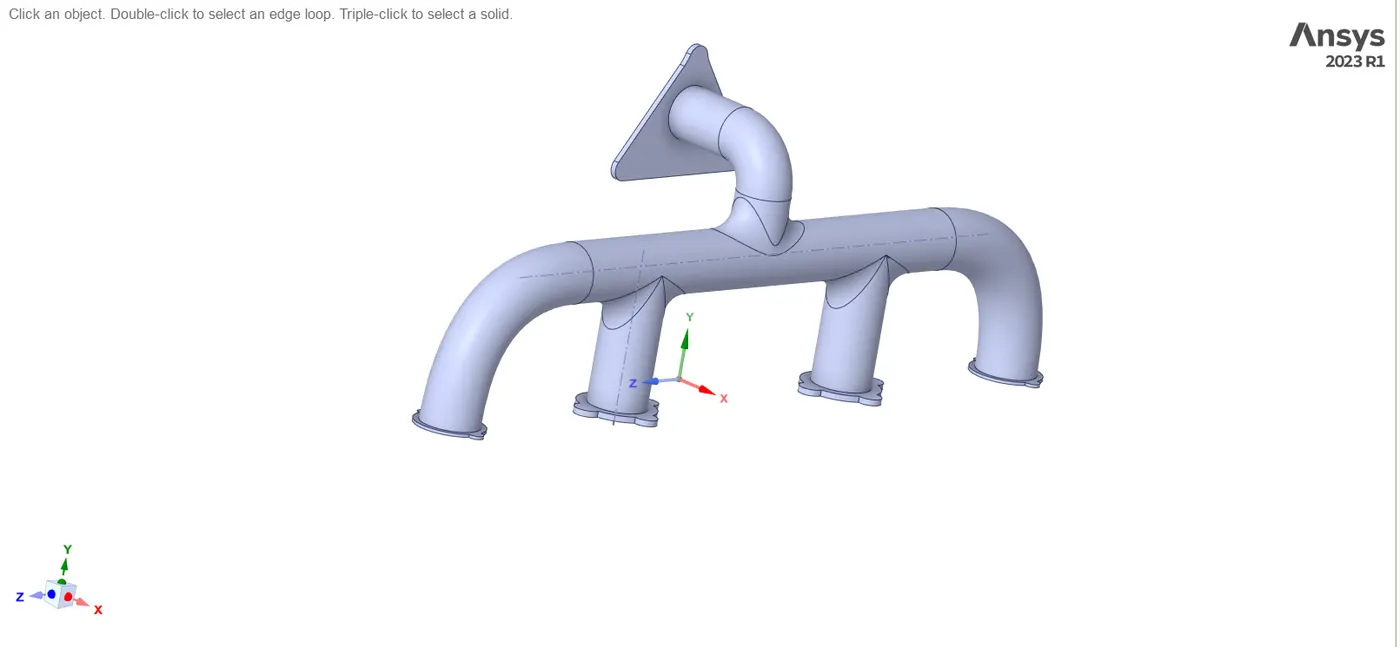
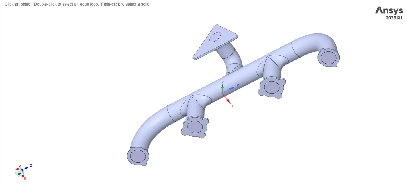
- The exhaust port was initially modeled in Spaceclaim.
- A three-dimensional representation was created, featuring four inlets and one outlet.
- Despite the presence of isothermal boundary conditions and a uniform flow rate at the four inlets, the model's asymmetry precluded dividing it into two halves for computational efficiency.
- The entire model was discretized to facilitate the subsequent meshing process.
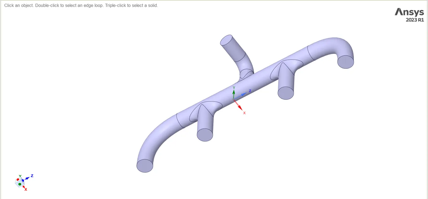
- For the Conjugate Heat Transfer (CHT) analysis, consideration of both solid and liquid volumes was necessary. Spaceclaim's volume extract feature was utilized to select edges for the fluid volume.
- Both the solid and liquid volumes were then duplicated into a single component.
- The establishment of a shared topology was a crucial step, ensuring mesh conformality between the fluid and solid volumes. Spaceclaim's "share coincident topology" option was selected and executed to achieve this, meeting the prerequisites for CHT analysis.
- Subsequently, the exhaust port was loaded into the meshing window and simulated for both baseline and refined meshes.
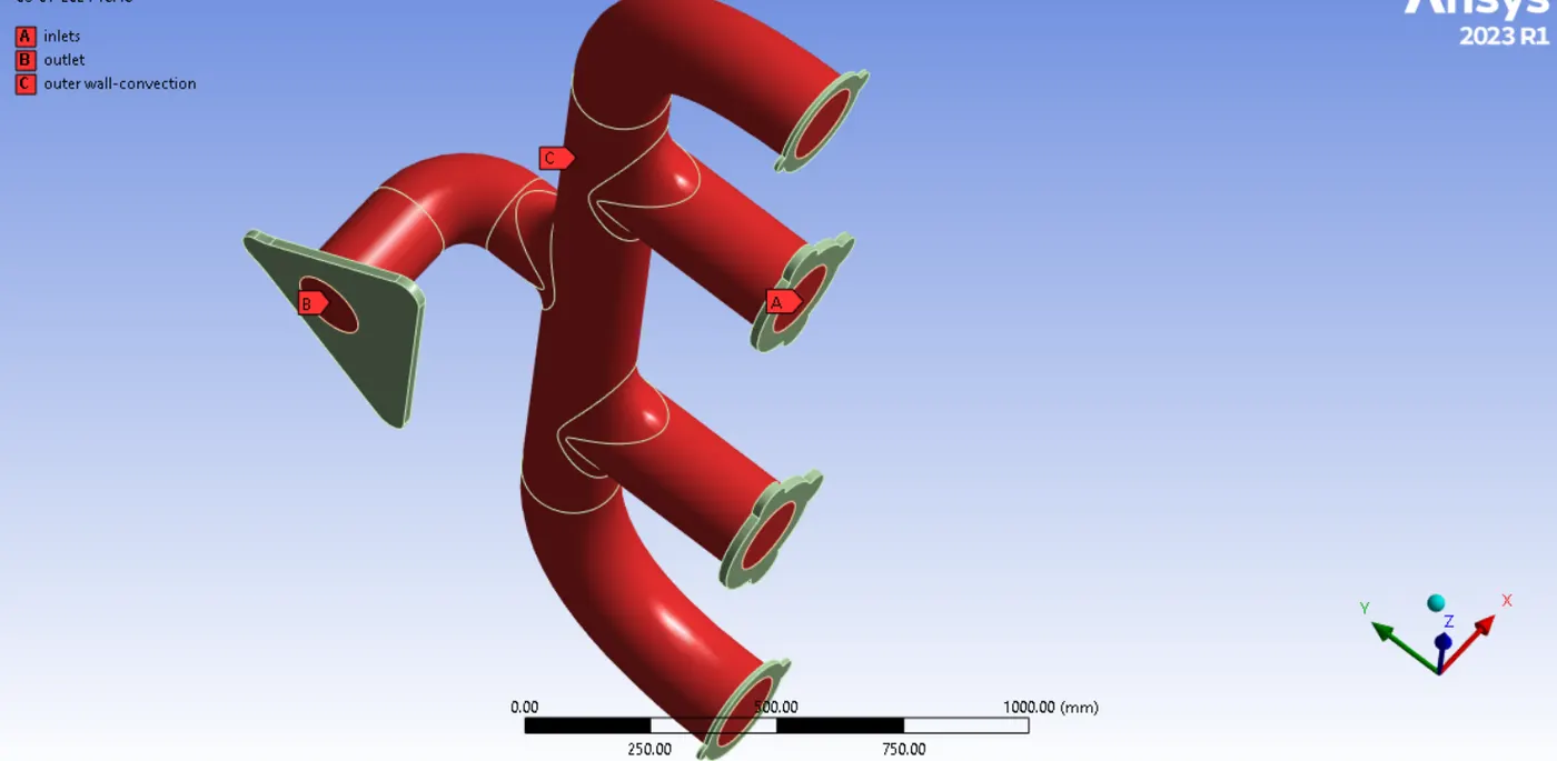
- Named selections were created to identify specific regions, including inlets, outlets, and outer wall convection.
- The analysis delved into the results by examining contour images and graphs. This comprehensive review aimed to grasp the behaviors of temperature, velocity, and surface heat transfer coefficients at the interface, providing valuable insights into the thermal dynamics of the system.
Open Mesh and name the components:
Inflation:
- Inflation layers facilitate the creation of a body-fitted mesh, aligning with the geometry.
- Essential at interfaces for accurate heat transfer calculations, capturing precise flow details.
- Start by selecting the fluid part and assigning it the name "inflation layer."
- In the global mesh, choose the inflation option. Use automatic inflation by selecting all faces in the chosen named selection.
- Specify the named selection for inflation by choosing the "inflation layer" created earlier.
- Determine the first layer thickness based on the desired `y^+' value and the turbulence model.
Freestream velocity: `U_(infty)`=5m/s
Freestream density: `rho`=1.225 kg/`m^3`
Dynamic viscosity: `mu`=0.000017894 kg/(m s)
Diameter of inlet: D=0.1662206 m
Desired `y^+`=1
Reynolds number:`Re = (rho ** U_infty ** D) / mu`=56896.2319 >4000 (Turbulent model)
Skin friction coefficient:`C_f = 0.026 ** Re^(-1/7)`=0.00544096214
Wall shear stress:`tau_(wall) = C_f ** rho **(U_infty^2) / 2`=0.08331473276
Friction velocity:`U_f = sqrt(tau_(wall) / rho)`=0.26079115541
First layer thickness:`Delta_s = y^+ ** mu / (U_f ** rho)`=0.0000560116653 m = 0.0560116653 mm
Insert the calculated total thickness,and maximum of 6 growth layers with growth ratio of 1.2.
- In this case, using the k-omega SST turbulence model, as `y^+' is between 0.1 to 5.
Turbulence Model - k-omega SST:
The k-omega SST turbulence model is a two-equation model that combines elements of both the k-epsilon and k-omega models. It is known for its versatility and ability to handle a wide range of flow conditions, from boundary layer flows to free shear flows.
This model is particularly suitable for simulating flows with adverse pressure gradients, separated flows, and areas with significant changes in flow direction.
CASE-1
Baseline simulation (without inflation layer)
element size =150mm
viscous model=SST-K-omega
inlet velocity =5m/s
inlet temperature=700k
HT co-efficient=20 `W/(m^2-k)`
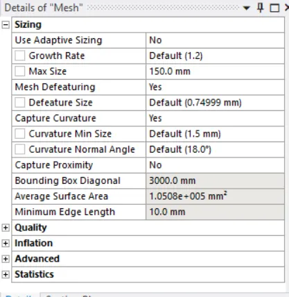
Mesh:
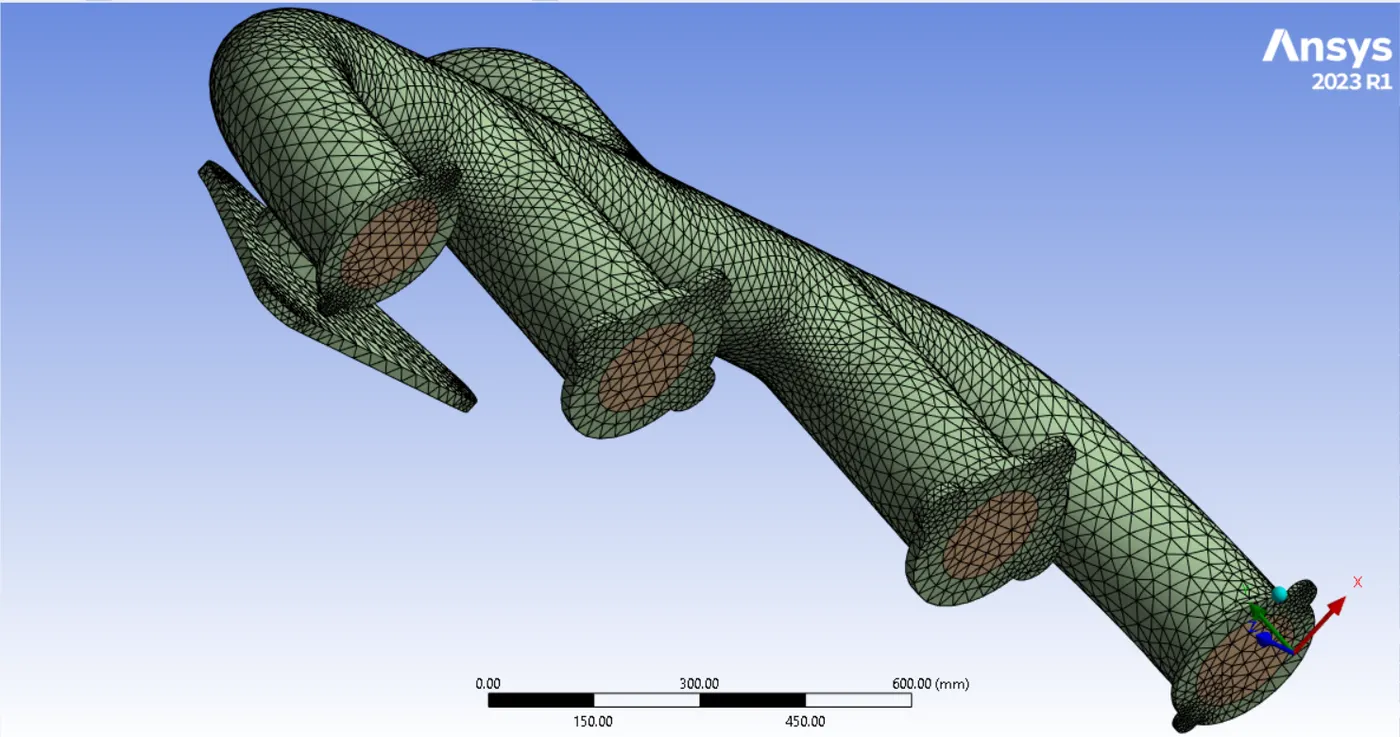
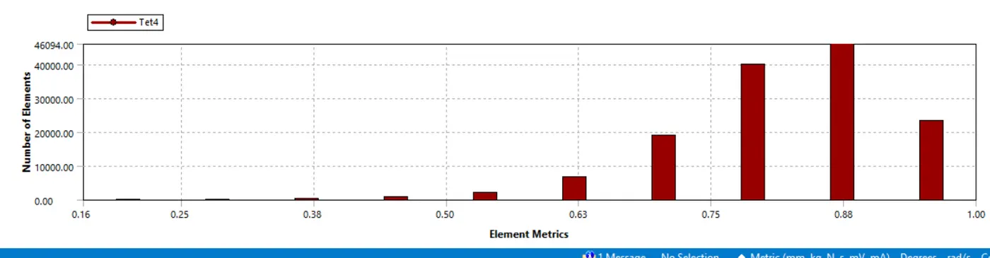
Mesh element quality is good:

Problem Setup :
- To set up our problem we open Fluent and setup inital conditions , boundary conditions material etc.,
- We first start with checking the mesh quality using perform mesh check under domain.If no error is seen in console window then we can proceed further.
- Then we move move to setting up physics where we select the solver ,viscous model ,initial and boundary conditions etc.,
- We use a steady state pressure based solver to solve our model.
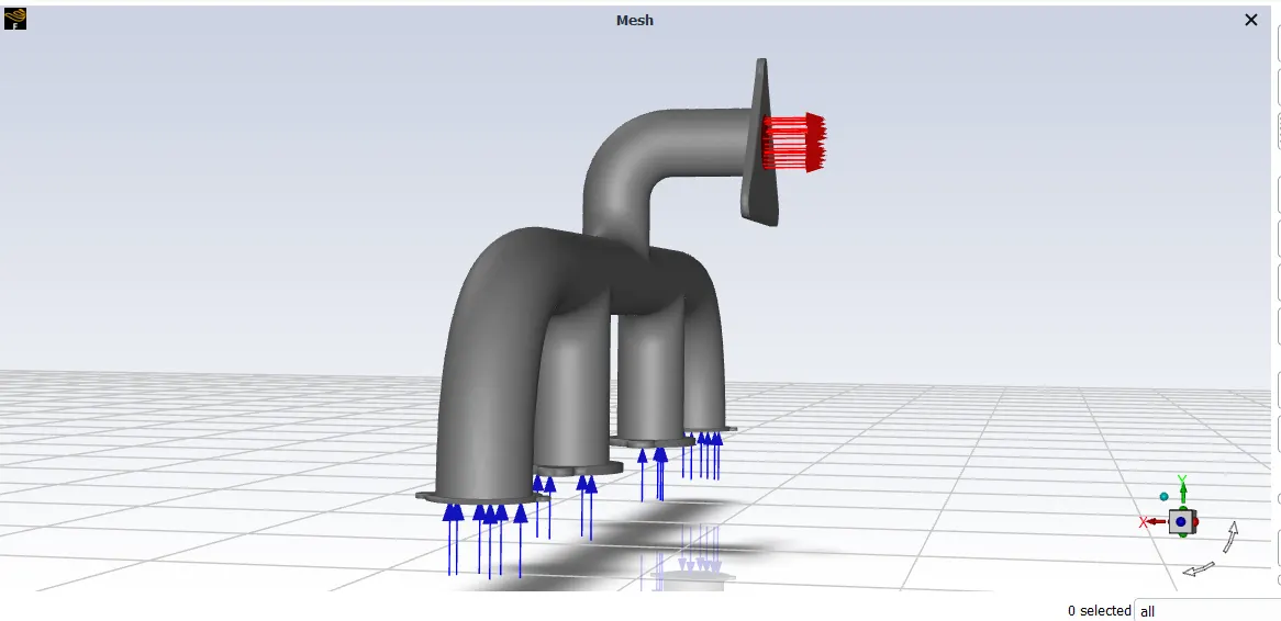
The different boundary conditions are listed below:
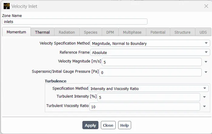
Inlet boundary condition
Type: Velocity inlet
Velocity magnitude : 5 `m/sec`
Temperature: 700 K
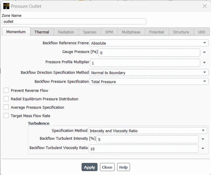
Outlet boundary condition
Type: Pressure outlet
Gauge pressure: 0 Pa
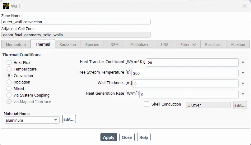
Outer wall convection
Type: wall
Thermal condition: convection
Heat transfer coefficient: 20 `W/(m^2K)`
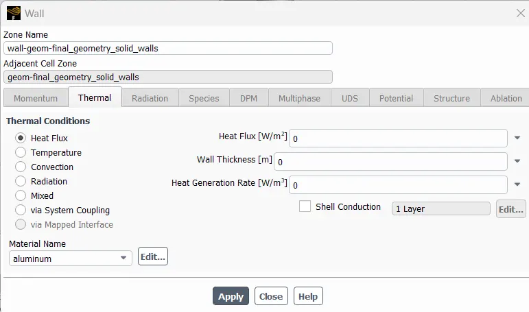
The rest boundary condition values are set up as default values in ANSYS-FLUENT.
Energy equation: enabled.
Viscous model: It is set to SST-K-omega
Material properties
Fluid
Material Name: Air
Density: 1.225 `kg/m^3`
Specific heat: 1006.43 `J/(kg K)`
Thermal conductivity: 0.0242 `W/(mK)`
Viscosity: 1.7894e−05 `kg/(m−sec)`
Solid
Material Name: Aluminium
Specific heat: 871 `J/(kgK)`
Thermal conductivity: 202.4 `W/(mK)`
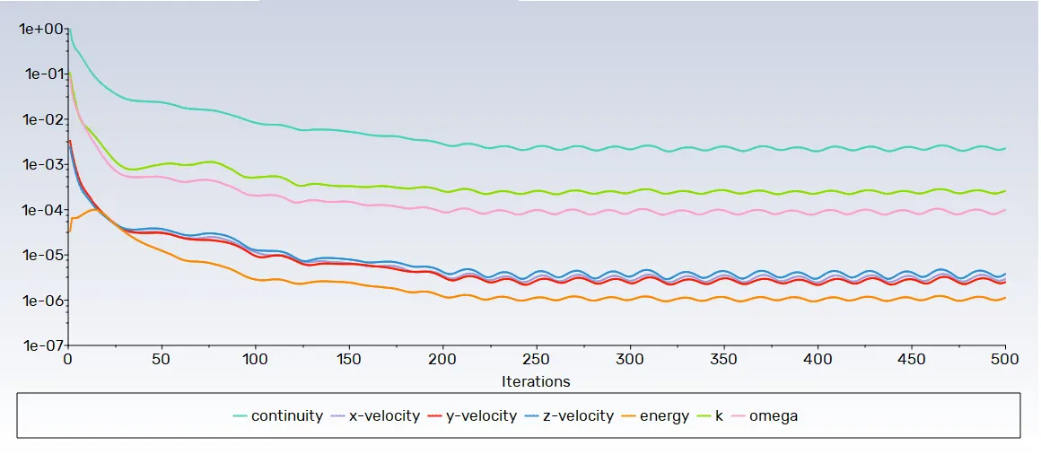
Residual Plot:
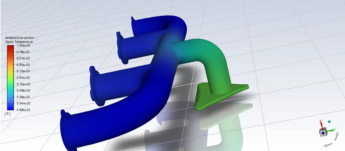
Temparature distribution:
surface heat transfer co-efficient:
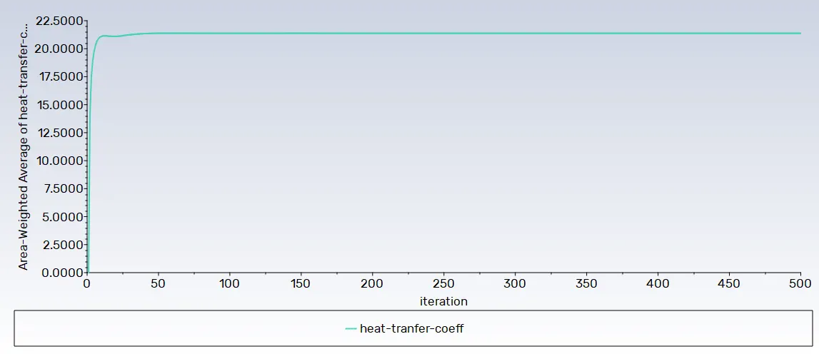
Heat transfer coefficient

CFD-POST results:
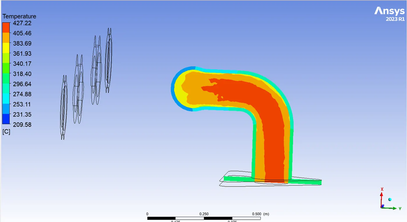
Temperature contour:
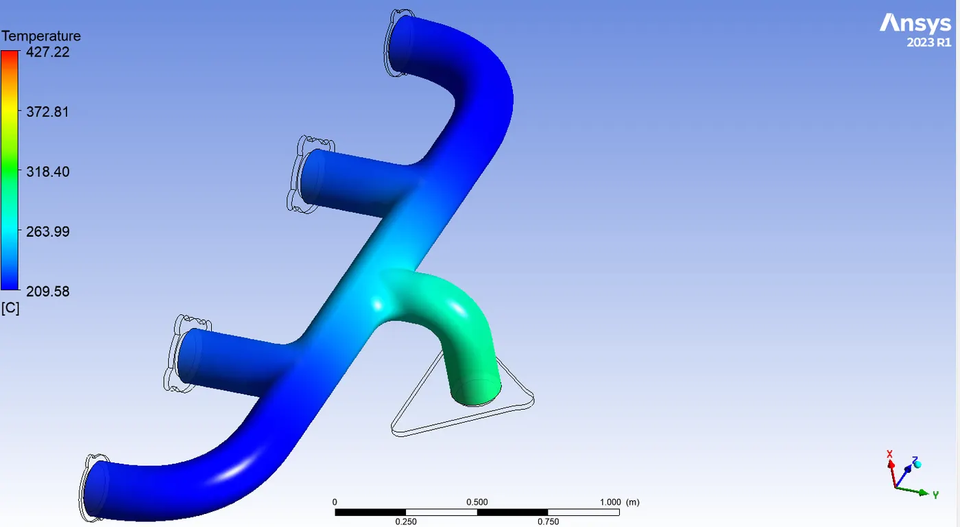
Temperature at exhaut outlet:
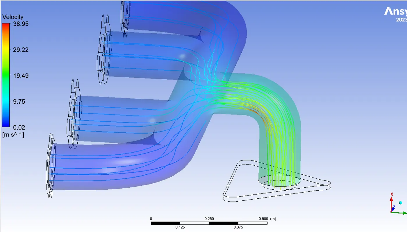
Streamline Velocity:
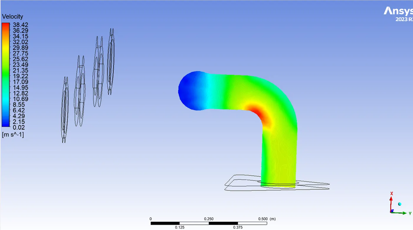
velocity contour at exhaust:
CASE-2
Element size =150mm
viscous model=SST-K-omega
inlet velocity =5m/s
inlet temperature=700k
HT co-efficient=20 `W/(m^2-k)`
Inflation layer:
Desired 'y^+`=1
First layer thickness: 0.0560116653 mm
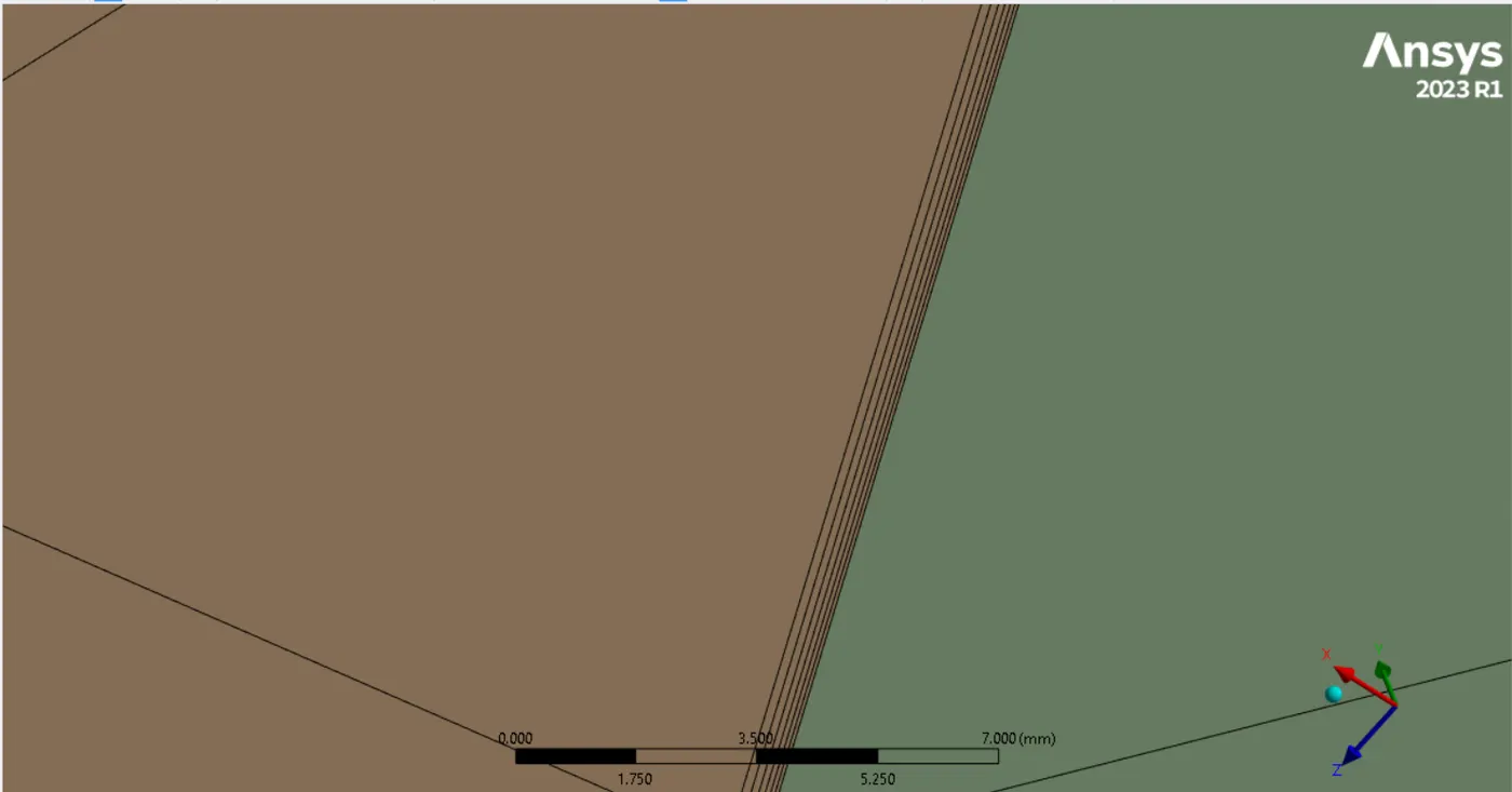
Mesh:
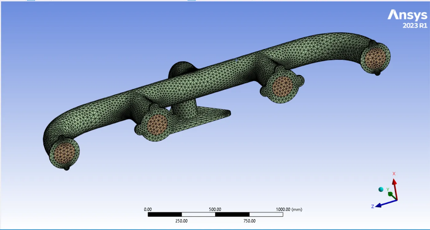
Using same stup method as used above for the baseline mesh, we get:
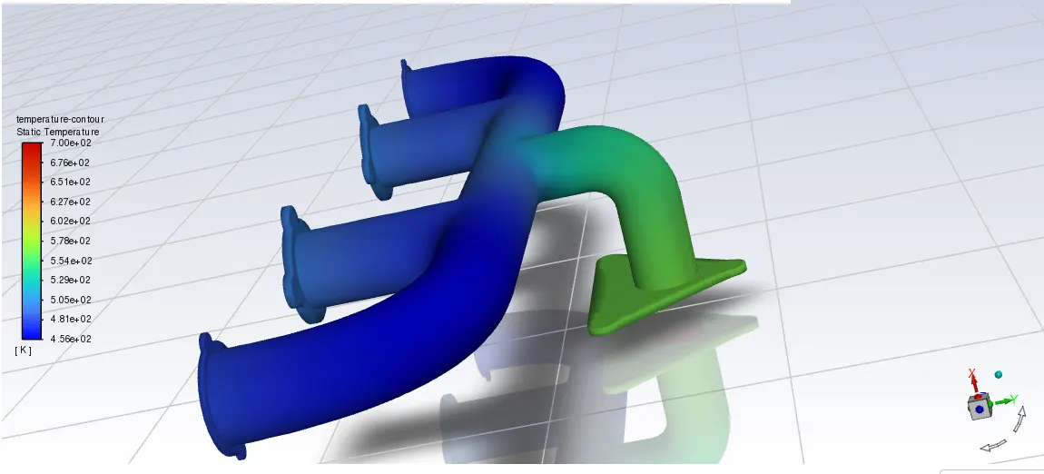
Temparature distribution:
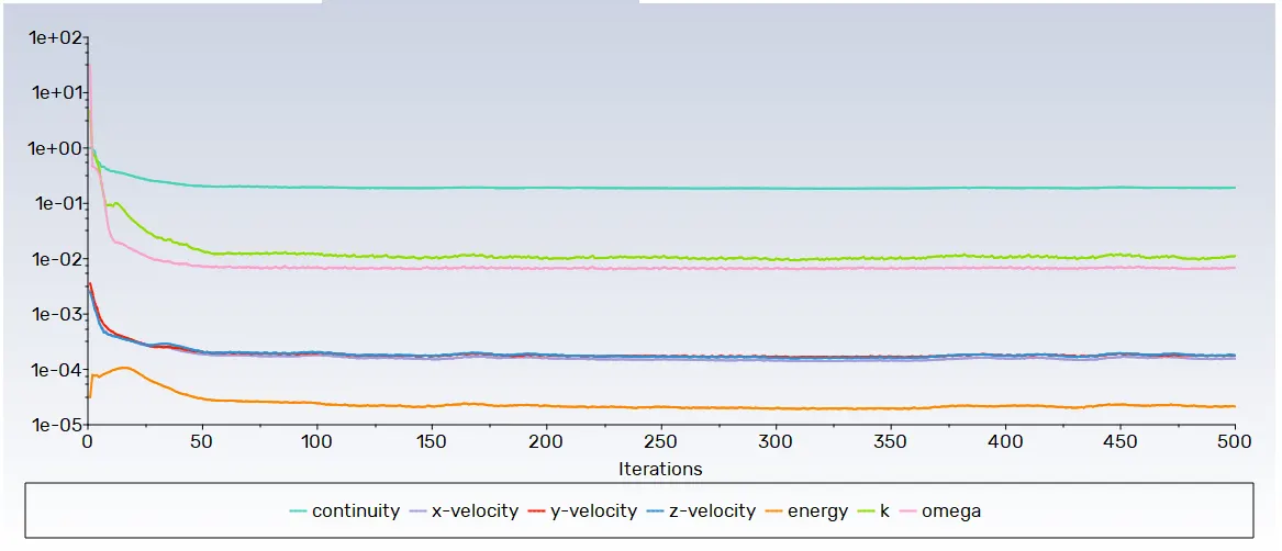
Residual plot:
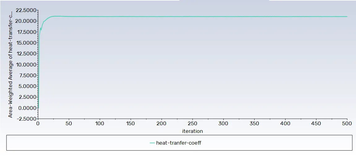
surface heat transfer co-efficient:

CFD-POST results:
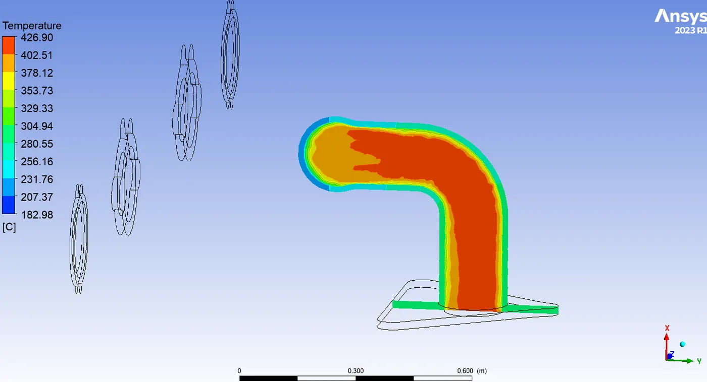
Temperature contour:
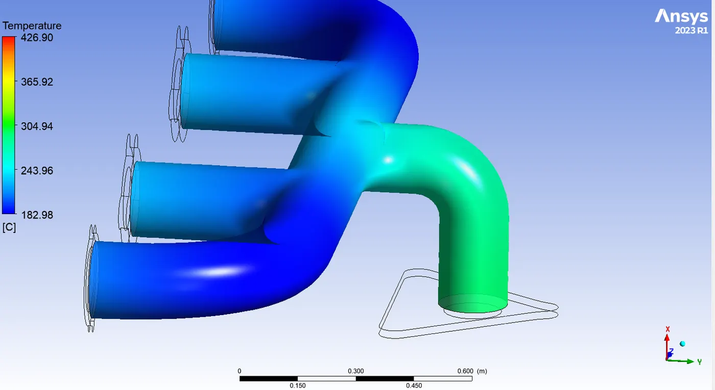
Temperature at exhaut outlet:
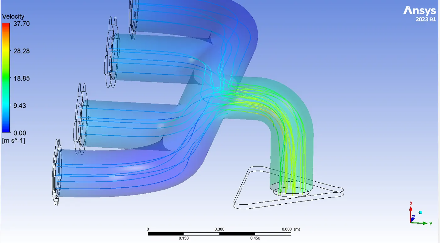
Streamline Velocity:
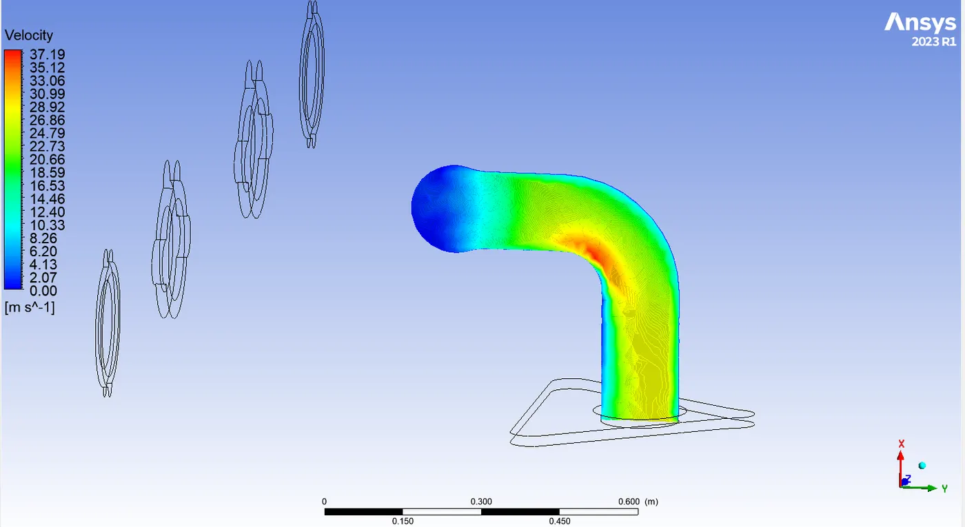
velocity contour at exhaust:
Case-3
Element size =90 mm
viscous model=SST-K-omega
inlet velocity =5m/s
inlet temperature=700k
HT co-efficient=20 `W/(m^2-k)`
Inflation layer:
Simulation with 'y^+`=1
First layer thickness: 0.0560116653 mm
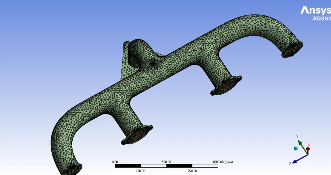
Using same stup method as used above for the baseline mesh, we get:
Temparature distribution:
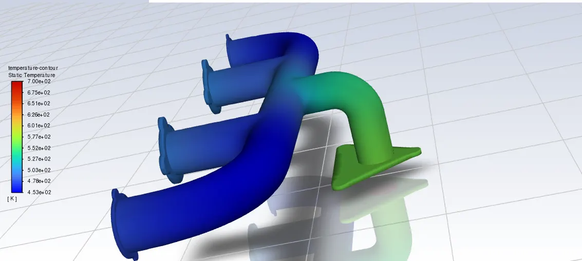
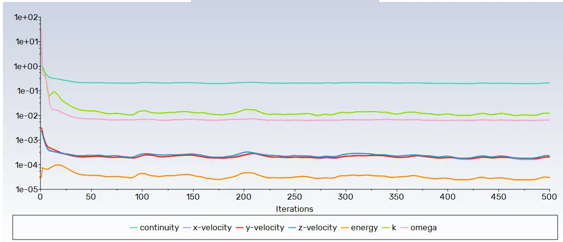
Residual plot:
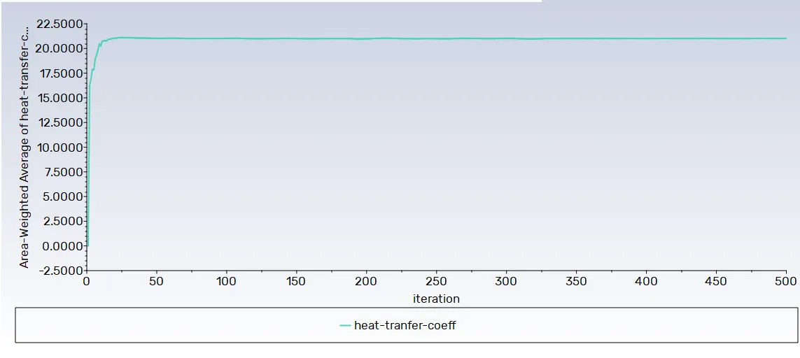
surface heat transfer co-efficient:

CFD-POST results:
Temperature contour:
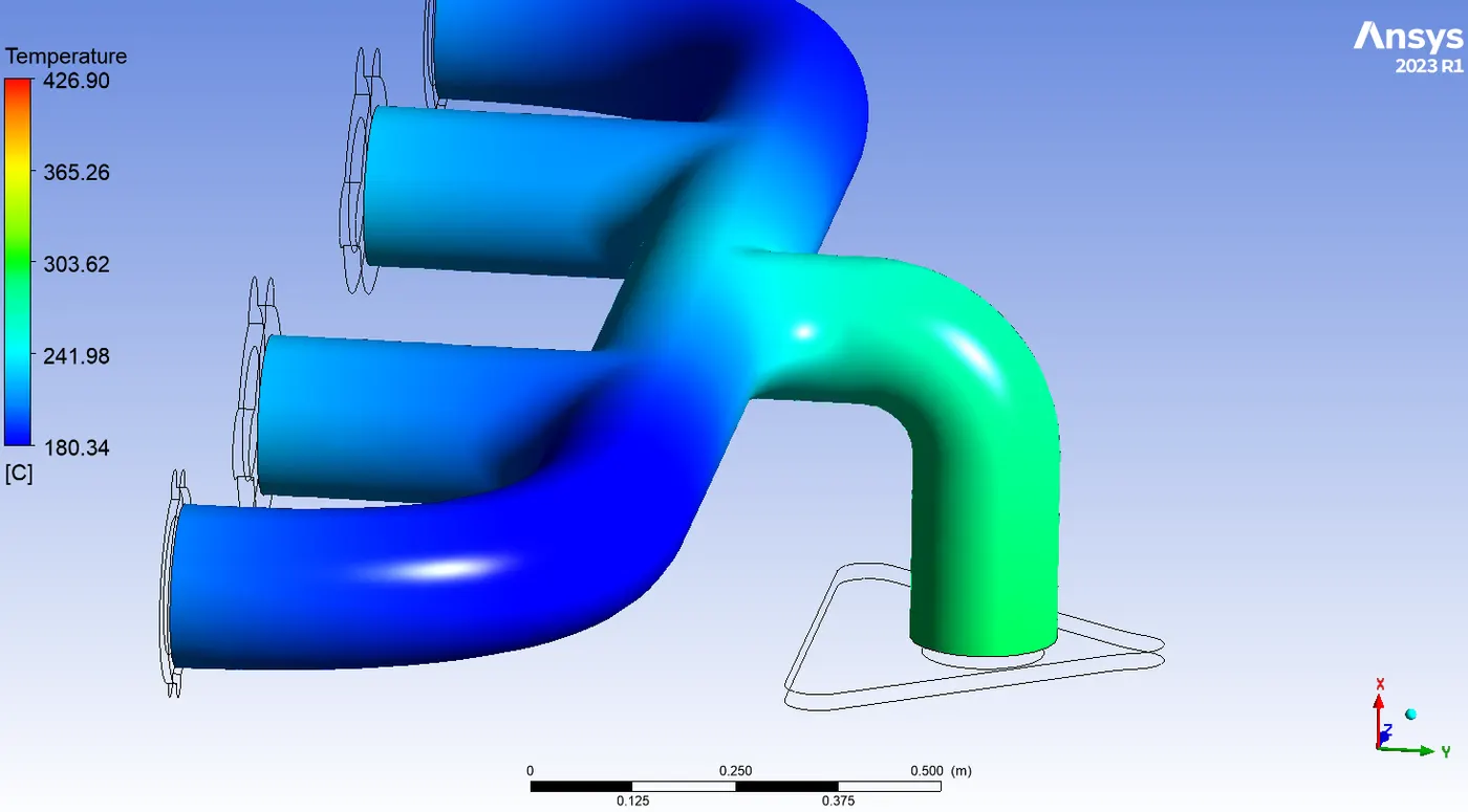
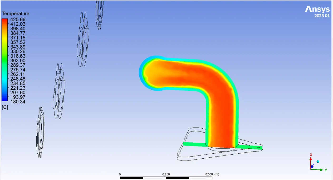
Temperature at exhaut outlet:
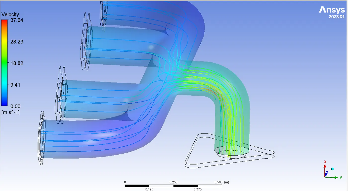
Streamline Velocity:
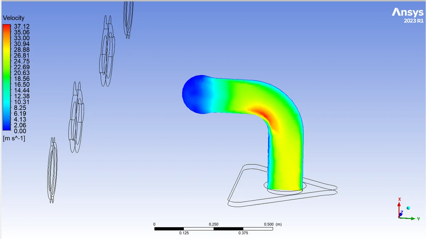
velocity contour at exhaust:
Case-4
Element size =50 mm
viscous model=SST-K-omega
inlet velocity =5m/s
inlet temperature=700k
HT co-efficient=20 `W/(m^2-k)`
fluid body sizing=30 mm
Inflation layer:
Simulation with 'y^+`=1
First layer thickness: 0.0560116653 mm
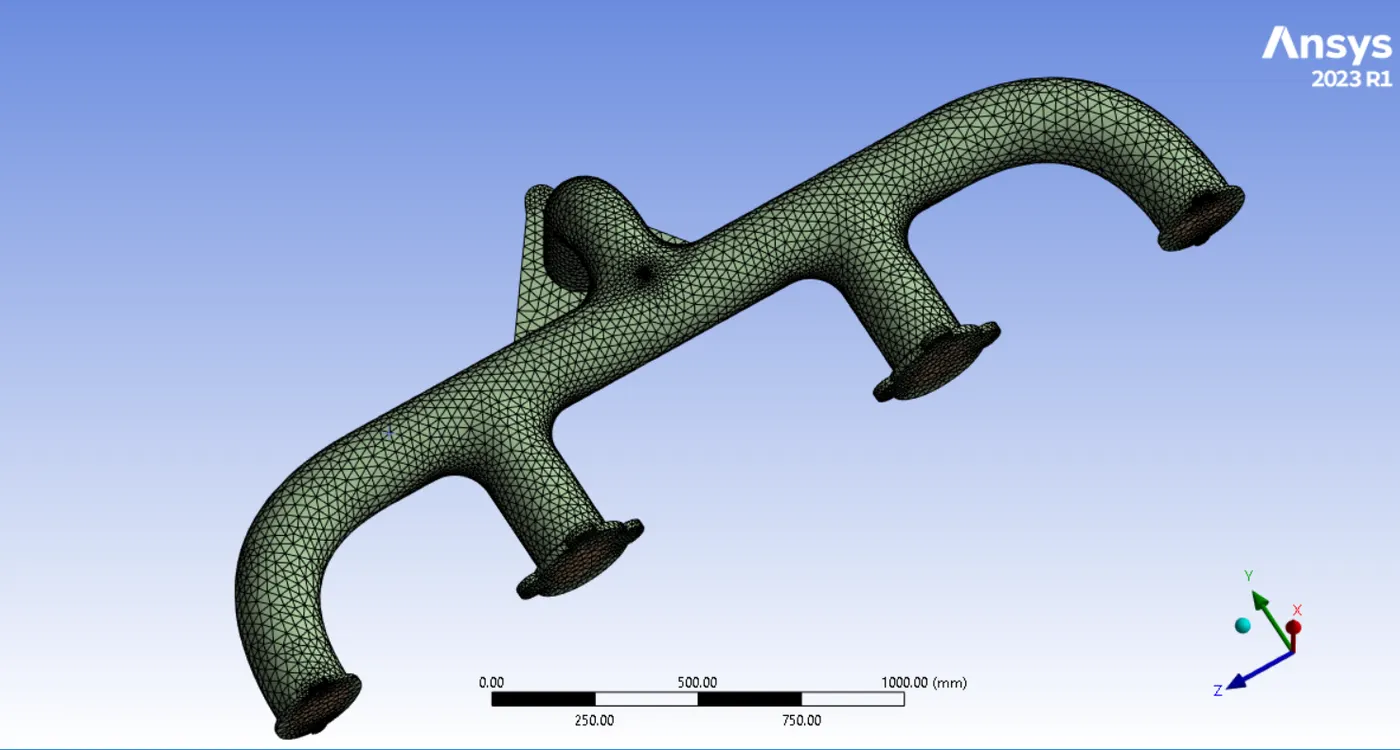
Using same stup method as used above for the baseline mesh, we get:
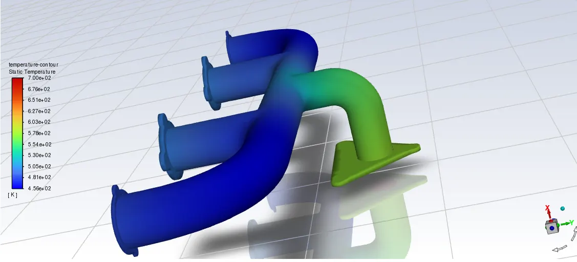
Temparature distribution:
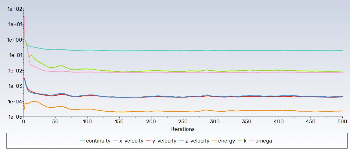
Residual plot:
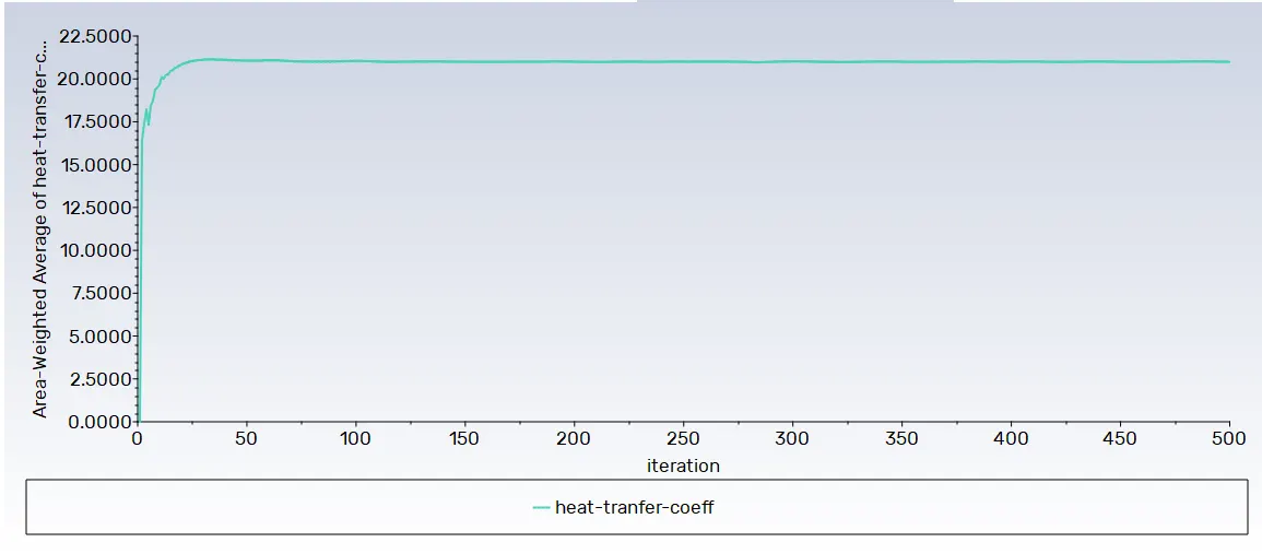
surface heat transfer co-efficient:

CFD-POST results:
Temperature contour:
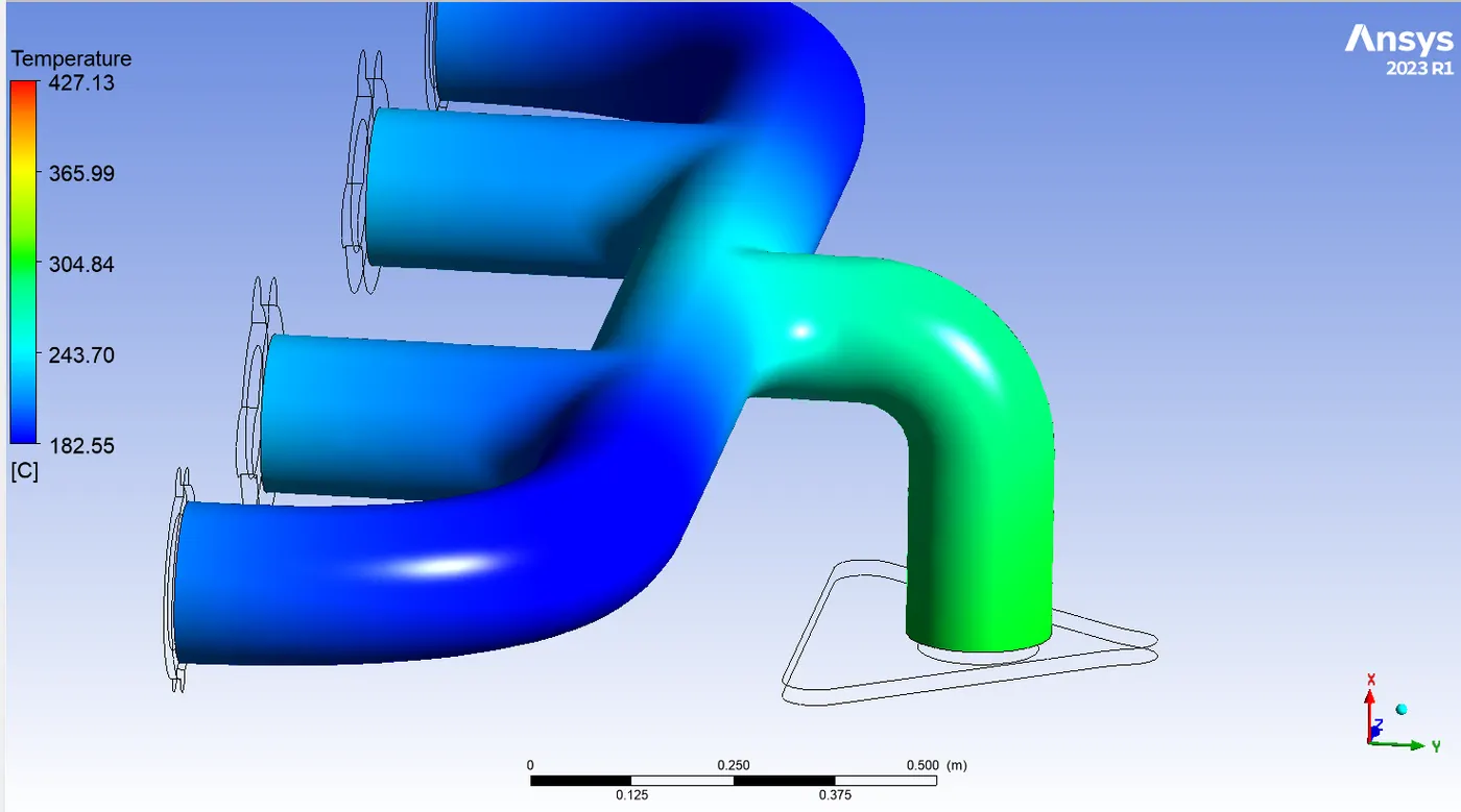
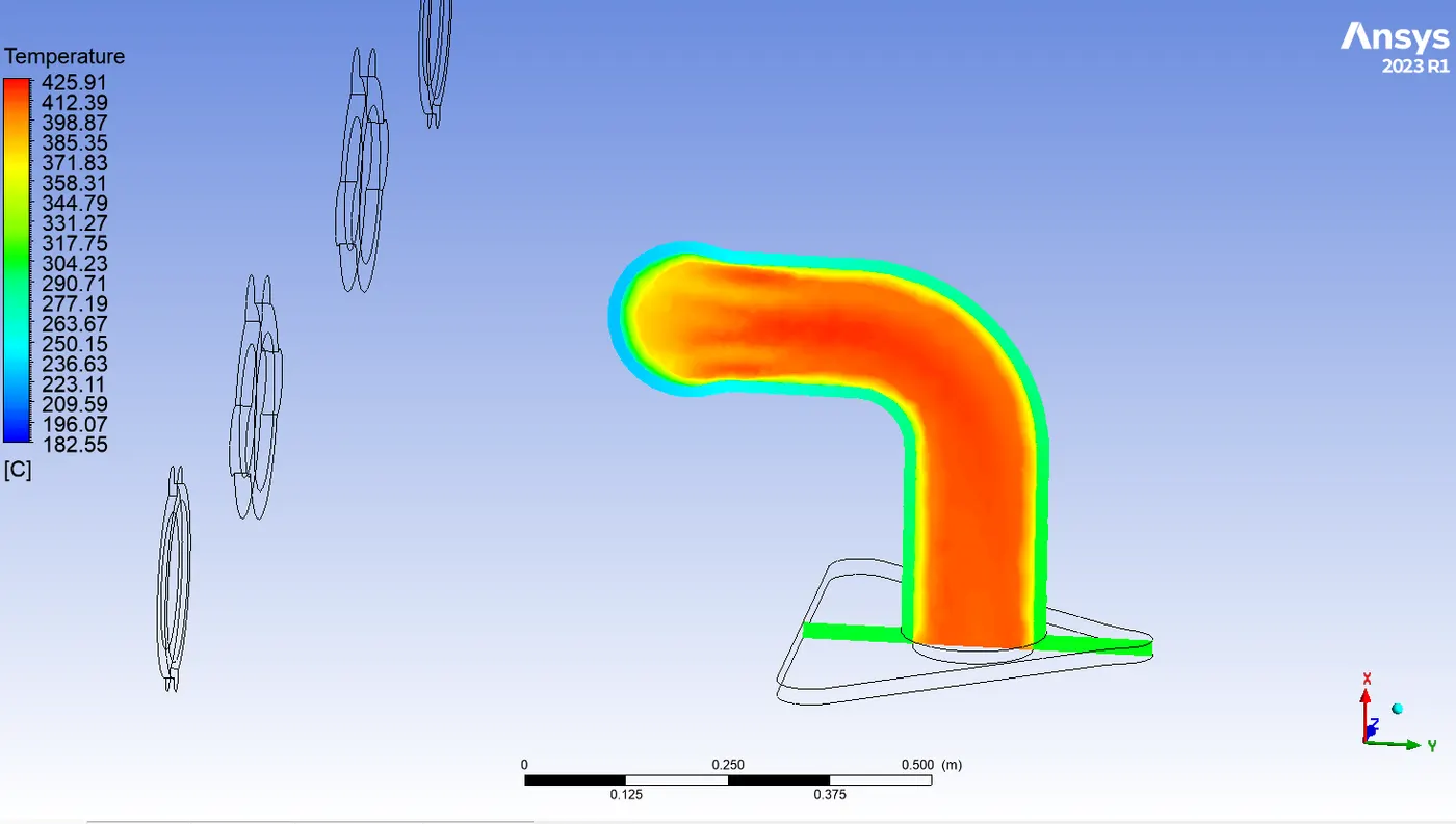
Temperature at exhaut outlet:
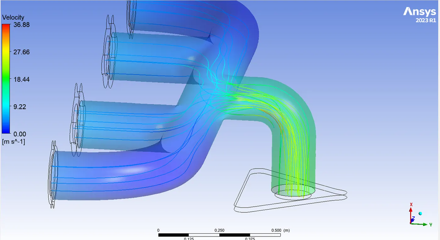
Streamline Velocity:
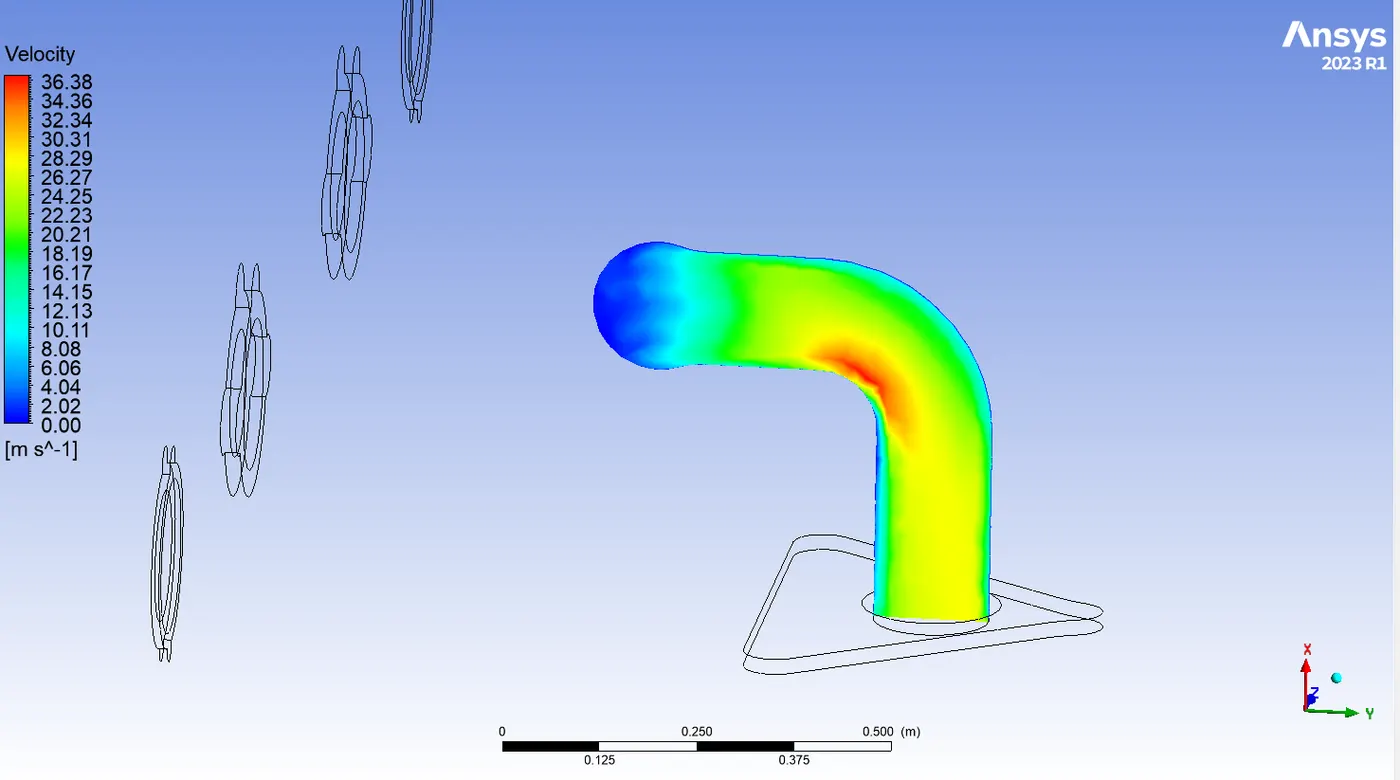
Velocity contour at exhaust:
Observation from the simulations:
- Velocity is lower at inlets compared to the outlet. Inlets have similar diameters, maintaining similar velocity.Volume flow rate (A*V) is conserved, resulting in very high outlet velocity.
- Higher outlet velocity leads to a higher Reynolds number and heat transfer coefficient.
- Streamline Plot: Velocity-colored streamlines illustrate the flow. Low velocity at inlets, significantly higher at the outlet due to mass conservation.Higher outlet velocity contributes to a higher Reynolds number and heat transfer coefficient.
- Heat Transfer Coefficient:Wall heat transfer coefficient calculated at the outlet walls adjacent to the fluid.Contour plot at outlet shows highest heat transfer at the curved section.Maximum heat transfer coincides with the highest velocity at the curved section.
- Fluid's high velocity at the curved section results in maximum heat transfer.
- Higher heat transfer coefficient at the curved section leads to elevated solid temperature.Fluid's high temperature at the outlet contributes to increased heat transfer to the solid.
---------------------------------------------------------------------------------------------------------------------------------------
In accordance with Bernoulli's mass conservation principle, the conservation of mass in our model is explicitly elucidated below.
Let's designate the flow rates from the inlets as Q1, Q2, Q3, Q4, respectively, and Q5 as the outflow from the exhaust manifold.
Given that mass is neither created nor destroyed, the mass flow rates are balanced, expressed as:
Q1+Q2+Q3+Q4=Q5...........................................eq(1)
Utilizing the equation
Q=ρ⋅A⋅V
(where ρ is density, A is the cross-sectional area, and V is velocity), Equation (1) transforms into:
A1⋅V1+A2⋅V2+A3⋅V3+A4⋅V4=A5⋅V5
In the context of incompressible flow, to maintain mass flow balance, velocity is increased. Consequently, overall mass flow rate is conserved.
Considering the high velocities, the Reynolds number at the outlet manifold is notably elevated.
For forced convection applications, the Nusselt number (Nu) is a function of Reynolds number (Re) and Prandtl number (Pr), expressed as Nu = f(Re, Pr).
Nu can also be defined as the ratio of convective heat transfer coefficient (h) to the thermal conductivity (k), i.e., Nu = hD/k.
Analyzing these equations, it is evident that Nu is proportional to Re and h. Thus, Re is directly proportional to h.
Our simulations reveal high velocities at the bend section of the outlet manifold, resulting in a higher Reynolds number, consequently leading to elevated heat transfer coefficients.
Hence, the predictions from our simulations can be deemed accurate.
Analytical solution
The Reynolds number for the given flow is 58189.8960, which suggests that the flow is turbulent in nature, the Dittus Bolter heat transfer coefficient relation can be used to determine the Nusselt number which is described mathematically as follows
`Nu_D=0.023**Re_D^(frac{4}{5})**Pr^n`
where `mu` is the dynamic viscosity of the fluid in `kg/(m−sec)`=1.7894e−05 `kg/(m−sec)`
k is the thermal conductivity of the material in `W/mK`=0.0242 `W/mK`
`C_p` is the specific heat capacity of the fluid at constant pressure= 1006.43 `J/(kgK)`
Therefore,
Pr=`μ∗Cp/k`= 0.74418
n is constant 0.3, heat transfer takes place from fluid to solid.
Therefore ,
`Nu_D`=136.4827
Therefore, convective heat transfer coefficient `h=Nu**k/D`=19.518 W/(m^2K)
| Case | Element size | Fluid body sizing | Number of elements | First cell height | `Y^+` | Inflation layer | Surface heat transfer coefficient.(Numerical value) | Surface heat transfer coefficient. (Analytical solution) | % Error |
| 1 | 150 mm | N/A | 137987 | N/A | N/A | N/A | 21.377185 | 19.518 | 8.6% |
| 2 | 150 mm | N/A | 209465 | 0.0560116653mm | 1 | 6 | 21.02338 | 19.518 | 7.2% |
| 3 | 90 mm | N/A | 209217 | 0.0560116653mm | 1 | 6 | 21.012261 | 19.518 | 7.1% |
| 4 | 50 mm | 30 mm | 209407 | 0.0560116653mm | 1 | 6 | 20.985416 | 19.518 | 6.9% |
Factors influencing the accuracy of Heat Transfer Coefficient (HTC) predictions include:
- Mesh Quality: A well-structured and fine mesh is crucial for capturing intricate flow patterns and temperature gradients accurately.
- Turbulence Model Selection: The choice of turbulence model, such as k-omega SST, affects the simulation's ability to represent turbulent flow characteristics accurately.
- Boundary Conditions: Accurate specification of boundary conditions, including inlet velocity, temperature, and other relevant parameters, is essential for realistic simulations.
- Convergence Criteria: The convergence criteria used during simulations impact the accuracy of results. Tightening convergence criteria can enhance accuracy but requires careful consideration of computational resources.
- Fluid-Structure Interaction (FSI): In scenarios where solid boundaries interact with fluid flow, incorporating FSI considerations becomes vital for accurate predictions.
CONCLUSION:
The Conjugate Heat Transfer (CHT) analysis on the exhaust port using ANSYS-FLUENT was successfully simulated, focusing on an inlet velocity of 5 m/s. The study aimed to achieve specific objectives, including understanding the applications of CHT analysis, ensuring alignment with the y+ value based on the turbulence model, and providing a rationale for the obtained results.
Key Findings:
- The pressure-based, coupled scheme solver in ANSYS-FLUENT effectively discretized the entire geometry for CHT analysis.
- The analytical value of the heat transfer coefficient was calculated as 19.4287 W/(m^2K).
- The deviation of numerical heat transfer coefficient values from the analytical solution ranged from 5% to 10% for the mesh refinements.These deviations were within compliance with industrial standards, indicating acceptable accuracy.
- The grid independence test during mesh refinement demonstrated that the values of the heat transfer coefficient for the second and final mesh refinements were close to each other.
- Choosing the second refinement was deemed suitable to balance computational time and project cost.
- The Y+ value was set to 1 (viscous sublayer), allowing for an accurate representation of the first cell height adjacent to the wall.
- The turbulence model used was k-omega SST. The presence of the boundary layer was evident near the inlet of the pipe, causing a no-slip condition due to viscous forces.
- The turbulent nature of the flow (Reynolds number 58189.8960) led to a transition in the velocity profile from flat to flutter, and the boundary layer vanished at the outlet.
- The velocity profile experienced changes from the inlet to the outlet due to variations in velocity. The outlet velocity being higher than the inlet was attributed to the presence of four inlets and one outlet, influencing the overall flow pattern.
Accuracy and Validation:
- The accuracy of the heat transfer coefficient depended on selecting a suitable Y+ value and the turbulence model (k-omega SST).
- Predicted heat transfer coefficient values were validated against numerical solutions, showing deviations in the range of 5% to 10%, aligning with industrial standards.
- Values predicted by the baseline mesh and the refined mesh were close, indicating that the boundary layer dynamics dominated at the outlet section of the exhaust port.
Recommendations and Future Considerations:
- Further Turbulence Model Exploration: Exploring other turbulence models may offer insights into the accuracy of predictions, especially in scenarios with complex flow characteristics.
- Sensitivity Analysis: Conducting sensitivity analyses on parameters like mesh size and turbulence model settings could enhance the understanding of their impact on results.