Week 2 - Flow over a Cylinder.

AIM:

To conduct a simulation of the flow over a cylinder to elucidate the Karman vortex street phenomenon.

PART-I:

To simulate the flow in both steady and unsteady cases, and compute the Strouhal Number for Re=100.

PART-II:

To calculate the coefficients of drag and lift for a cylinder at Reynolds numbers of 10, 100, 1000, 10000, and 100000 using a steady solver and discuss the impact of Reynolds number on the coefficient of drag. Ensure that the results are validated against established literature, with errors within a 5% margin.

Expected Results:

• Demonstrate flow convergence in both approaches, identifying key quantities or plots indicative of convergence.
• Provide plots depicting the coefficients of drag and lift.
• Present plots illustrating vortex shedding patterns behind the cylinder.
• Include a reference to the preferred material, such as a relevant paper or Fluid Mechanics textbook, at the conclusion of the challenge submission page.

Introduction:

The study of fluid flow around bluff bodies, particularly circular or rectangular cylinders, is a classical problem in fluid mechanics with broad engineering applications. This investigation holds significance in various fields, including heat exchangers, chimneys, and the assessment of hydrodynamic loading on marine piles, offshore platform risers, and support legs.

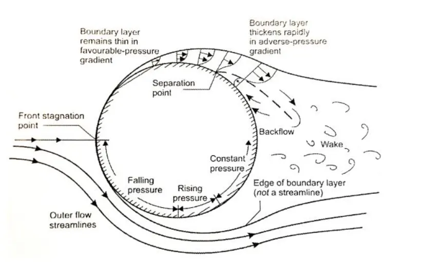
From a scientific standpoint, the flow around a circular cylinder exhibits key fluid dynamic phenomena, including the transition to turbulence, separation points, and vortex shedding. The flow characteristics over a circular cylinder surface can be observed in the diagram, highlighting the formation of boundary layers, points of separation, and wake formation.

Reynolds Number and Flow Patterns:

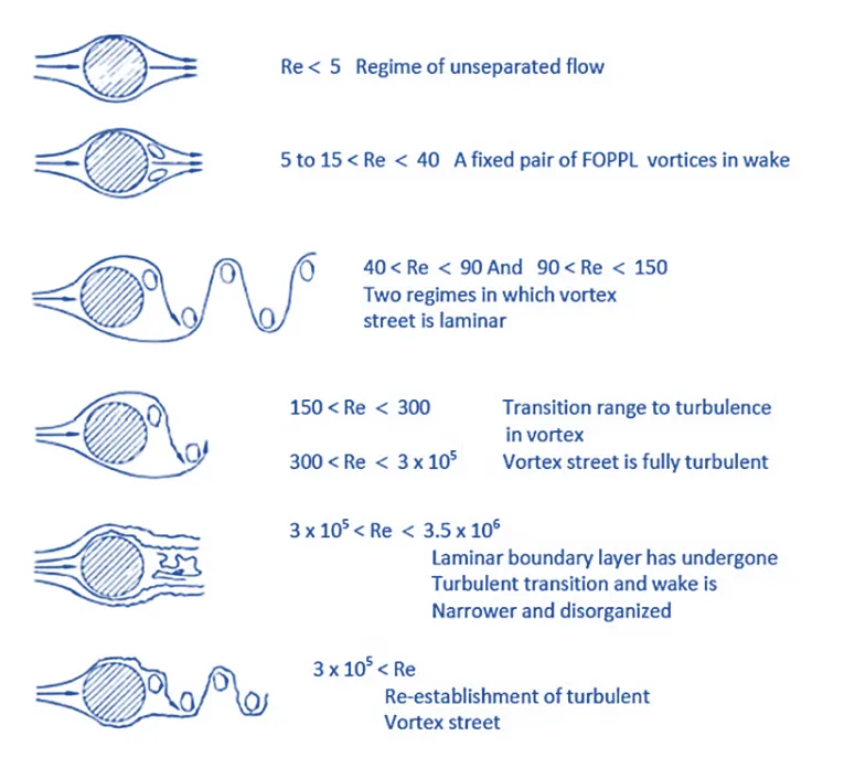
The Reynolds Number serves as a crucial parameter dictating the flow behavior around objects. Different ranges of Reynolds Numbers correspond to distinct flow patterns.

Low Reynolds Numbers (Laminar Flow):At low Reynolds Numbers, the flow pattern is characterized as laminar, exhibiting smooth and constant fluid motion. This is indicative of orderly and streamlined flow around objects.

High Reynolds Numbers (Turbulent Flow):Conversely, at higher Reynolds Numbers, the flow pattern becomes turbulent. This is marked by chaotic eddies, vortices, and flow instabilities. Turbulent flow is associated with more complex and irregular fluid motion.

Example in Nature: This behavior is exemplified in various natural phenomena, where low Reynolds Numbers may depict the calm and ordered flow of a gentle stream, while high Reynolds Numbers showcase the turbulent chaos seen in the swirling motion of a rapid river or turbulent clouds.

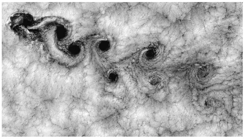
Turbulent Von Karman Vortex flow of Cloud

Strouhal Number:

The Strouhal number is a dimensionless number describing oscillating flow mechanisms. It represents the ratio of inertial forces due to the local acceleration of the flow to the inertial forces due to the convective acceleration.

`St = f . D / V `

where,

f = frequency of vortex shedding.

L = characteristic length (for example, hydraulic diameter or the airfoil thickness).

U = flow velocity.

Solutions:

The simulation of the flow over a 2D cylinder is a complex endeavor with various fluid properties requiring monitoring. The resulting flow exhibits the Karman Vortex Street pattern, a distinct oscillatory phenomenon observable in practical scenarios. Understanding this pattern is crucial for interpreting the outcomes of the simulation.

In simpler terms, the flow around a cylinder, when in motion at a constant speed in a fluid at rest, undergoes distinct phases. At very small Reynolds numbers, the flow is entirely laminar, devoid of recirculation or instability. As Reynolds numbers increase, a recirculation zone emerges behind the cylinder, marked by two eddies with opposite signs closely trailing the cylinder. With further increases in Reynolds numbers, these eddies become unstable and progressively depart from the cylinder, propagating in the wake to form the characteristic "Von Karman" vortex street.

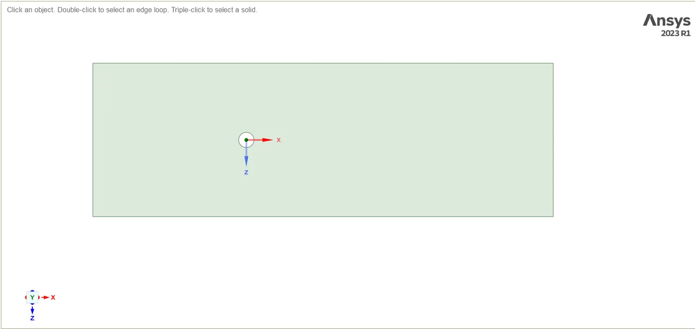
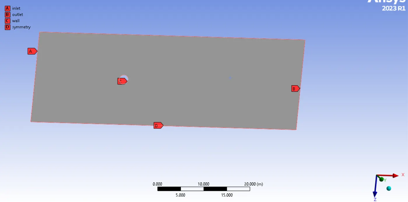
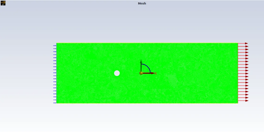
We used line tool to draw with dimensions

circle - 2m, with circle origin - -20 on X and +40 on X-axis.

box - 60x20m

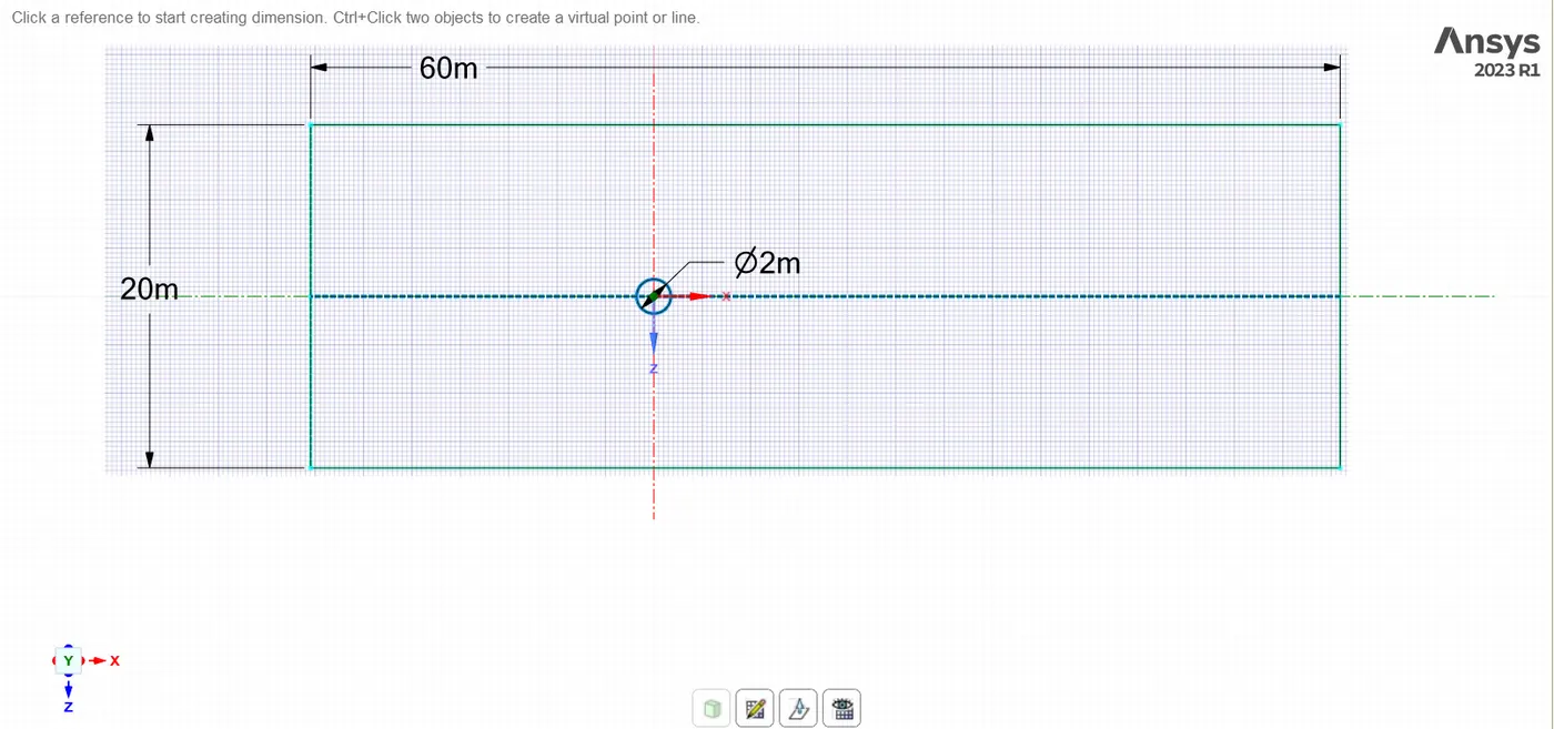
and then used Pull to create a surface from the geometry that looks like

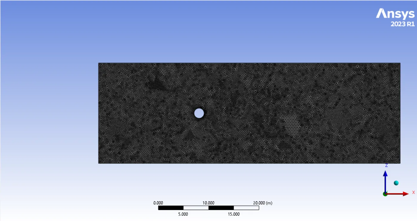
The subsequent phase involves mesh generation. Our goal is to attain a finely detailed triangular mesh, necessitating specific steps to ensure its desirability. Various methods and tools will be employed for this purpose. The following outlines the steps involved in the process. The existing mesh is referred to as the "former mesh."

Though we are going to have undesirable physical simulation at the CFD post with this amount of MESH as we performed beforehand what elements size is suitable for that physical phenomenon.

So we further tuned it more to finer mesh with an element size of 0.25 mm and we have

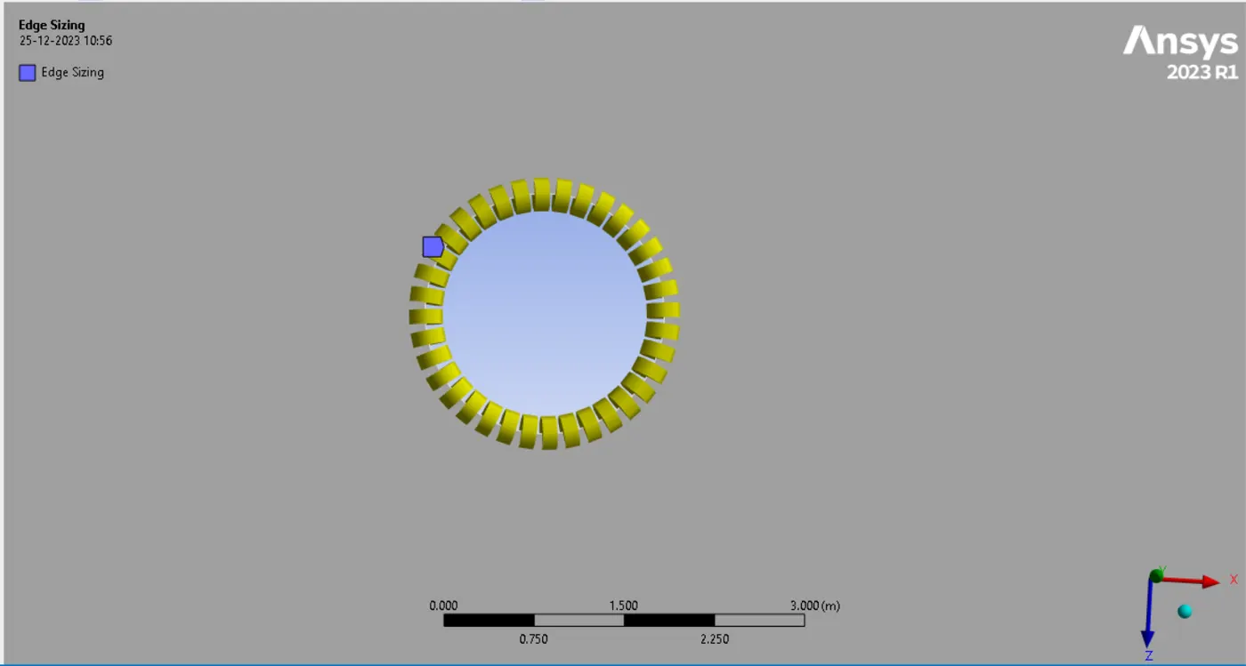
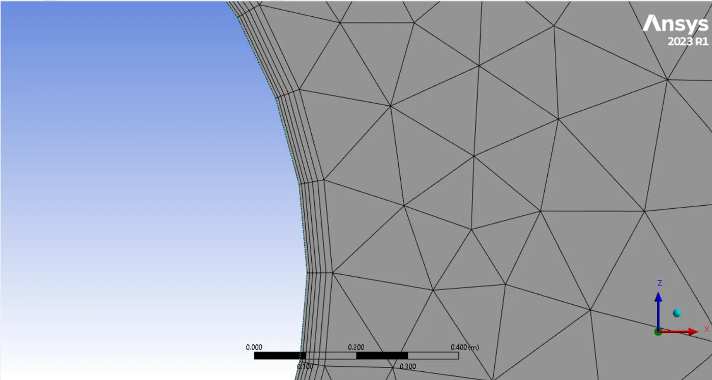
Moreover, for determining the element sizing, a more refined cylinder layer is introduced. This refinement involves increasing the number of edges by 36, ensuring that each edge is separated by 10 degrees from one another.

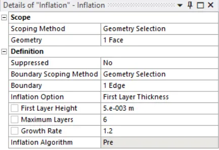
The same goes for the inflation layer.

Fluent Setup:

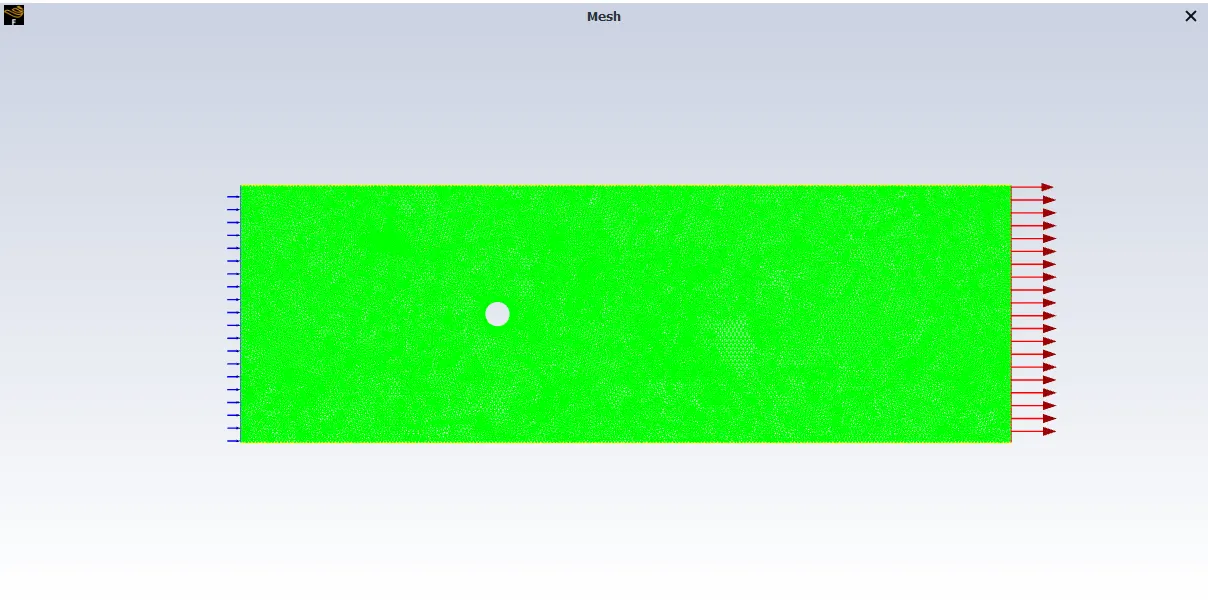
As a preliminary step, execute the "Check Mesh" operation to identify and rectify any potential errors in the geometry.

For this simulation focused on vortex shedding induced by flow over a cylinder, it is imperative to configure the physics parameters in alignment with the flow characteristics. Key parameters for vortex shedding include fluid material density and viscosity. Introduce a new material profile into the Fluent database to accurately represent the required fluid properties for this simulation.

General setup:

• Solver- Pressure Based.
• Velocity formulation- Absolute.
• Time- Based on the case study we are going to do (Steady/Unsteady).
• 2D Space- Planer

Materials:

Create/Edit- user-material (The fluid is created such that only viscosity will be resopnsible for varing Reynold's number.)

Name- user-material

Properties- Density (kg/m3)= 1 (constant)

Viscosity (kg/m-s)= 0.02 (constant)

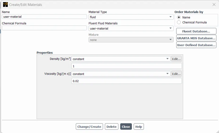
To check the vortex nature it is important to know the Reynolds no.

Reynolds Number:

The Reynolds number is a measure of the ratio of inertial to viscous forces in the flow of a fluid and may be defined as:

`Re = ρVD/ μ`

where:

`rho` = Density,

D = the diameter of the cylinder around which the fluid is flowing,

V = the steady velocity of the flow upstream of the cylinder and

`mu` = the kinematic viscosity of the fluid.

By applying the Reynolds number, fluid viscosity, fluid density, and cylinder diameter, we can determine the magnitude of flow velocity, as explained in the Reynolds Number theory mentioned above.

Boundary Conditions:

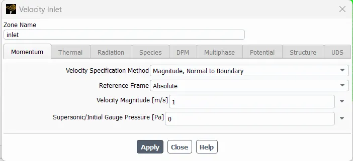
Inlet- Velocity Inlet

Velocity Magnitude for:

Inlet velocity(U) -

Re = UL/nu

U = Re*(mu/rho)/L

U = 100*(0.02/1)/2

U = 1 m/s

• Re = 100--->1 m/s

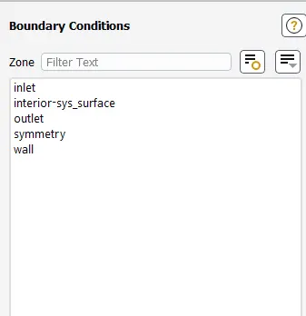
Velocity inlet:

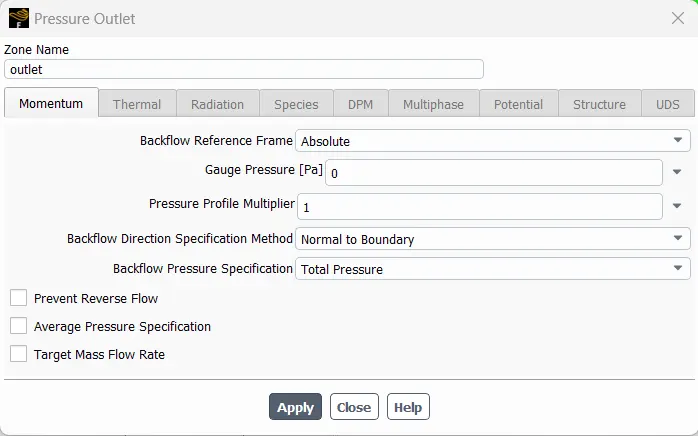
Outlet- Pressure outlet

Gauge Pressure- 0 Pa

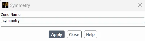
Symmetry:

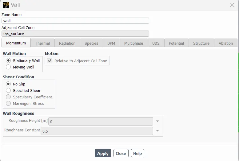
Wall:

Report Definations

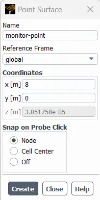
Generate a surface report defining the vertex average of velocity magnitude at a monitoring point situated 8m away to the right of the cylinder's center along the X-direction.

Report Definitions:

To read a average velocity value at above monitor point go to Report definitions - surface report - vertex average.

Coefficient of Drag and Coefficient of Lift report created using force report.

For drag go to definations - new - force report - Drag

For lift go to definations - new - force report - Lift

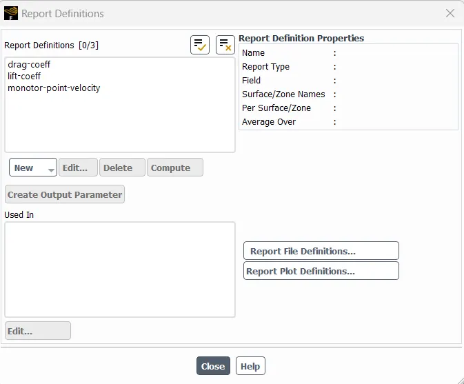
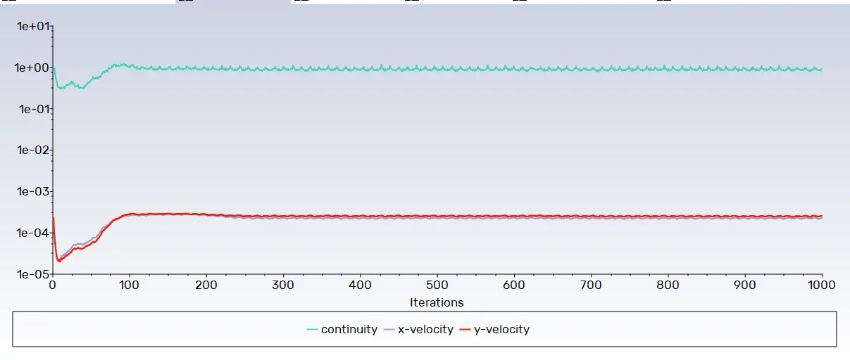
For both steady and unsteady state simulations, the following plots are to be presented:

1. Residual Plot: This plot provides insights into the convergence points, indicating when convergence is achieved.
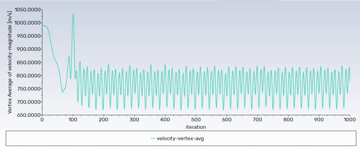
2. Monitor Point Velocity Plot: A monitor point, positioned 8m from the cylinder, is utilized to calculate the velocity at that specific point.
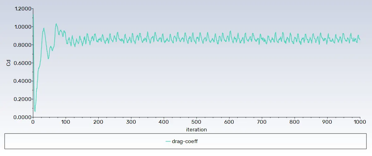
3. Drag Coefficient Plot: Illustrates the drag coefficient calculation.
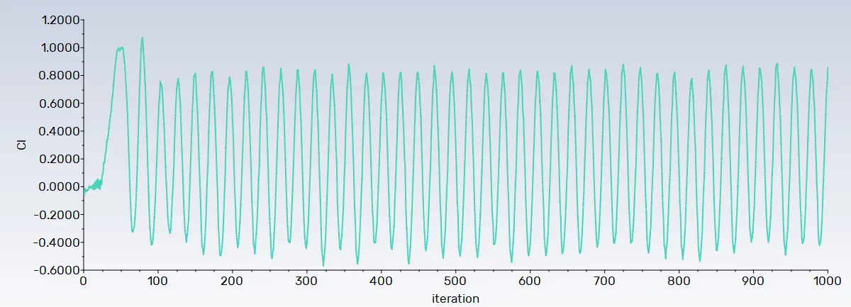
4. Lift Coefficient Plot: Displays the lift coefficient calculation.
5. Velocity Contour Plot: Offers a visualization of velocity variations in the flow over the cylinder.
   
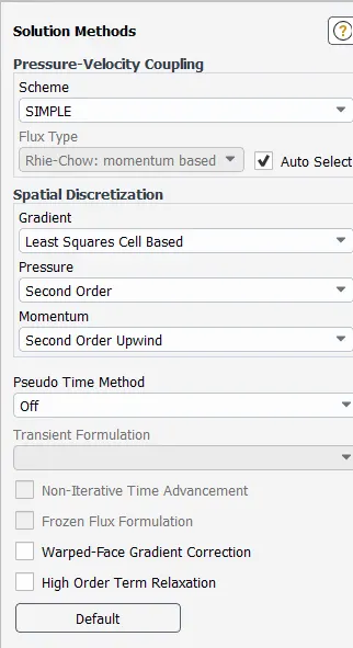
   Initialization Method:
   Hybrid for STEADY STATE simulations
   Standard for UNSTEADY STATE simulations
   
   
6. Contour Plots of Pressure & Velocity: Reveals the distribution of velocity and pressure, providing a comprehensive view of the flow characteristics.

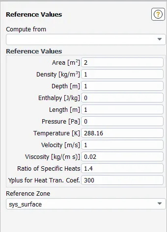
Reference Values was set to:

Run calculation:

Setup parameters :

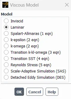
Viscous model - Laminar

Solver type - Pressure based

Solving Scheme - SIMPLE

Initializing method - Hybrid(for Steady case)

Standard(for Transient case)

No. of Iterations - 1000

Drag and Lift:

In aerofoil shapes, the direction of drag and lift forces is crucial. When a body moves through a fluid, it encounters resistance, akin to the sensation experienced by extending one's arm out of a moving car window. Forces and moments may be exerted by a fluid on a body in various directions. The force exerted by a flowing fluid on a body in the flow direction is termed drag.

In a stationary fluid, only normal pressure forces act on the immersed body's surface. However, in a moving fluid, tangential shear forces arise due to the no-slip condition caused by viscous effects. The drag force results from the combined effects of pressure and wall shear forces in the flow direction. The components of these forces in the direction normal to the flow induce movement in that direction, and their sum is referred to as lift.

The magnitude of drag and lift forces relies on factors such as fluid density (`rho`), upstream velocity (V), and the body's size, shape, and orientation. Instead of listing these forces for various situations, it is more practical to work with dimensionless numbers representing drag and lift characteristics. The drag coefficient (`C_D`) and lift coefficient (`C_L`) are these dimensionless numbers, defined as follows:

Here,

`C _D ​ =( 0.5*ρ*V ^2* A)/ F _D ​`

`C _L ​ =( 0.5*ρ*V ^2* A)/ F _L`

`F_D` and `F_L` are the drag and lift forces,

`rho` is the fluid density,

`V` is the mean velocity,

`A` is the projected area (product of thickness and diameter of a cylinder).

These coefficients are particularly insightful as they depend only on the Reynolds number and the object's shape, irrespective of its size.

Workflow:

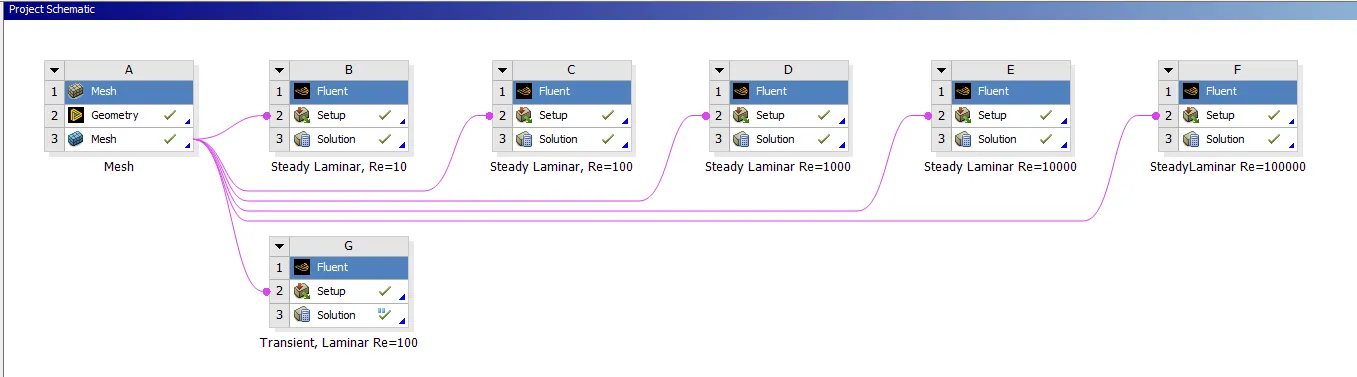
PART-I: Simulating Flow and Calculating Strouhal Number

In this phase, the flow will be simulated under both steady and unsteady conditions, with a specific focus on calculating the Strouhal Number for Reynolds number (Re) equal to 100.

For Unsteady State a slight modification has been introduced in the simulation. Standard initialization is carried out with a specified time step, as detailed in the setup description.

Steady State Flow For Re = 100:

The steady-state flow simulation will be executed for Reynolds number (Re) equal to 100.

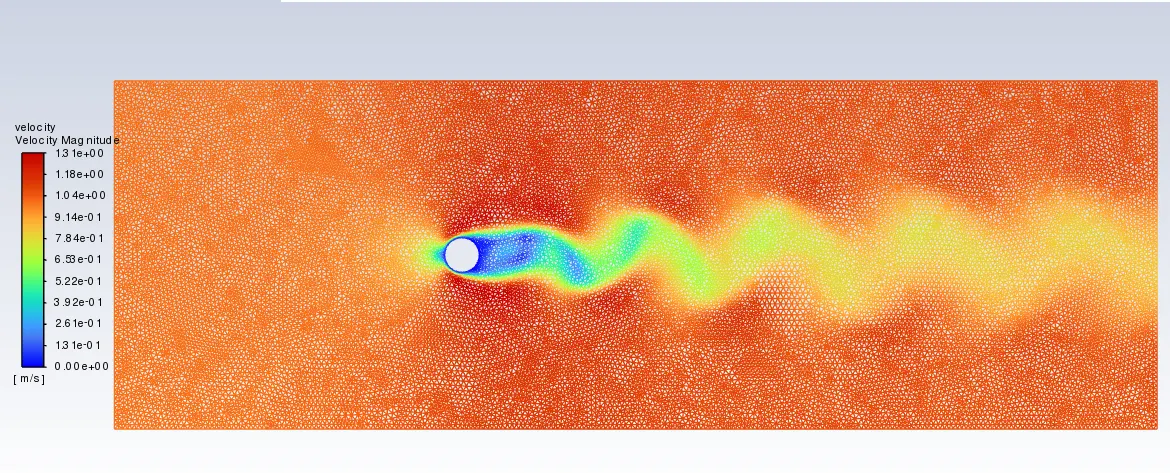
Fig - Velocity Contour For Re = 100(Steady)

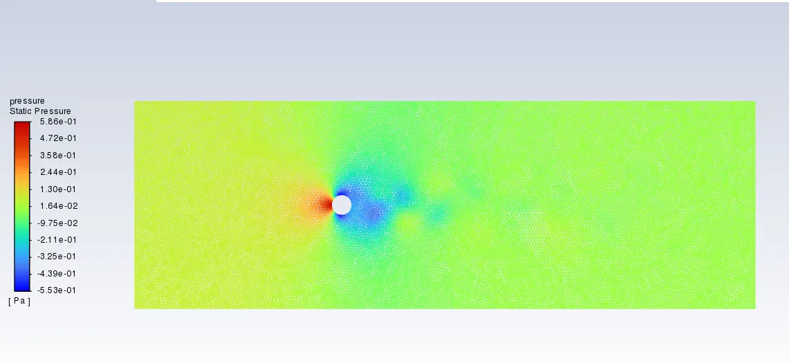
Fig - Pressure Contour For Re = 100(Steady)

Unsteady State Flow For Re = 100:

The unsteady-state flow simulation will be executed for Reynolds number (Re) equal to 100.

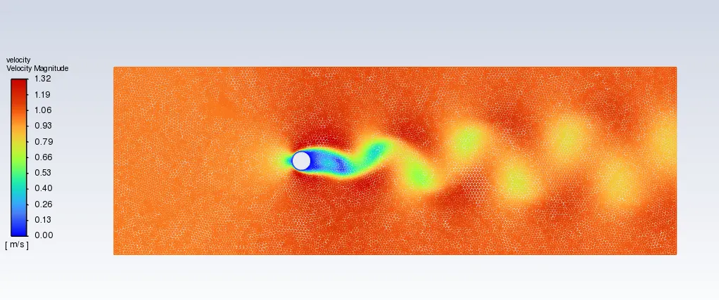
Fig - Velocity Contour For Re = 100(Transient)

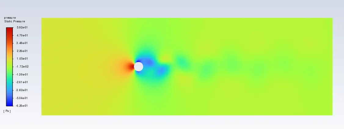
Fig - Pressure Contour For Re = 100(Transient)

Now lets compare the results of both the cases -

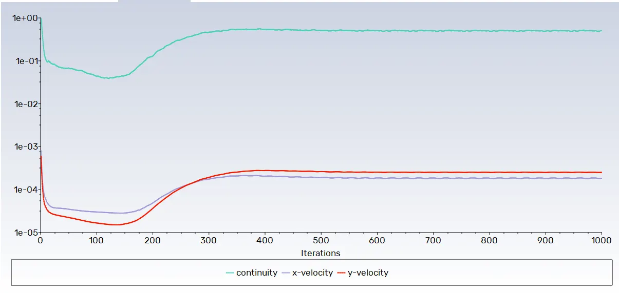
Fig - Residual Plot For Re = 100(Steady)

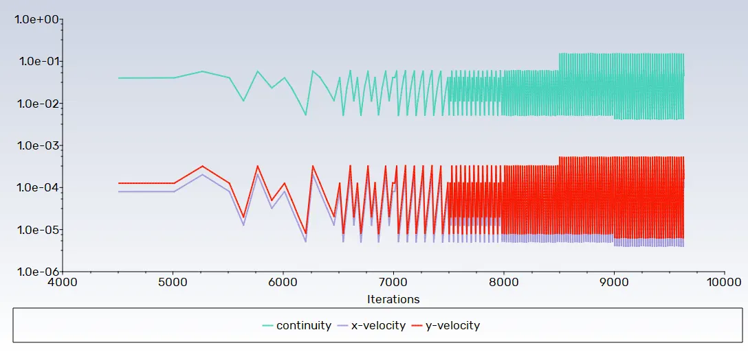
Fig - Residual Plot For Re = 100(Transient)

Analysis of Residual Plots and Convergence:

Upon scrutinizing the residual plots, it is evident that significant differences exist between the steady and transient cases. In the steady-state solver, it can be affirmed that the solution converges after approximately 370 iterations.

However, in the transient case, pinpointing the exact convergence point solely based on the residual plot is challenging. To decisively ascertain solution convergence, additional parameters are essential. Therefore, a monitor point is strategically positioned at 8 meters in the wake of the cylinder to calculate a key metric (velocity). This approach allows us to assess if repeated results with the same frequency are obtained, providing confidence in the convergence of results. The monitor point results serve as a crucial indicator of solution convergence in the transient case.

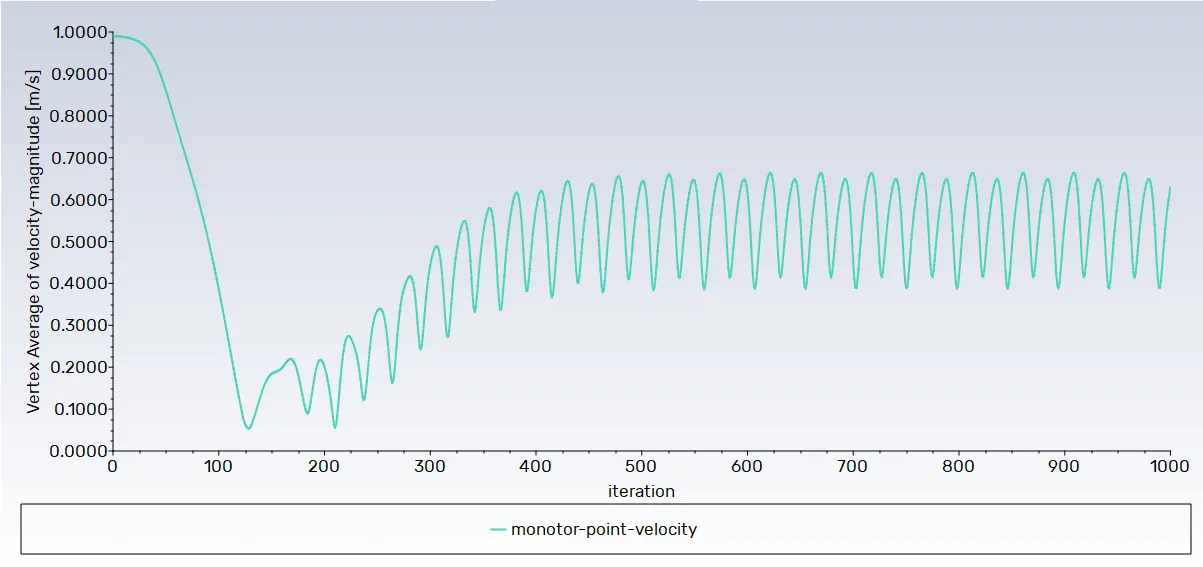
Fig - Vertex Average of Velocity Magnitude Plot For Re = 100(Steady)

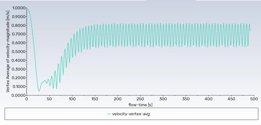
Fig - Vertex Average of Velocity Magnitude Plot For Re = 100(Transient)

Analysis of Monitor Point Results:

In the initial graph, it is observed that the frequency of velocity repeats after approximately 450 iterations. This observation leads to the conclusion that the solution has converged for the steady case.

Contrastingly, in the transient simulation, the velocity frequency remains constant and is expected to increase over time. This behavior indicates the evolving nature of the solution in the transient case, with the velocity frequency exhibiting a consistent pattern.

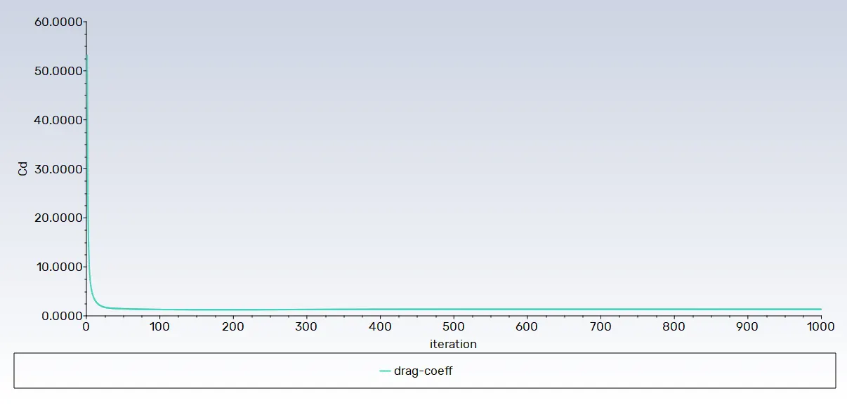
Fig - Coefficient of Drag Plot For Re = 100(Steady)

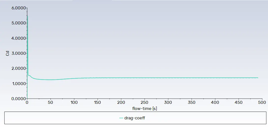
Fig - Coefficient of Drag Plot For Re = 100(Transient)

Comparison of Drag Coefficients:

When comparing the steady and transient cases based on their drag coefficients, a distinct pattern emerges. In the steady state, the drag coefficient stabilizes and remains nearly constant after approximately 100 iterations. However, in the transient case, the drag coefficient exhibits slight variations.

Despite the fluctuations in the transient case, both solutions converge to the same value of drag (1.3). This consistency in the drag coefficient values across steady and transient simulations indicates the reliability and agreement of results between the two approaches.

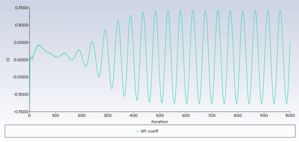
Fig - Coefficient of Lift Plot For Re = 100(Steady)

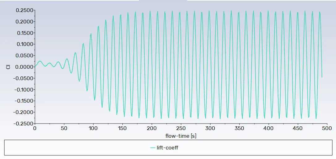
Fig - Coefficient of Lift Plot For Re = 100(Transient)

Analysis of Lift Plot:

In the lift plot comparison, distinctive characteristics are observed between the steady and transient solutions. In the steady solution, the frequency of lift improves gradually from zero to approximately +/-0.15. This suggests a systematic increase in lift frequency over time.

On the other hand, in the transient solution, a repeating sine wave pattern is evident. The lift values exhibit a periodic oscillation, indicating a consistent and repetitive behavior in the transient simulation from +/-0.237.

These differences in lift behavior highlight the dynamic nature of lift forces in both steady and transient flow scenarios.

Strouhal Number

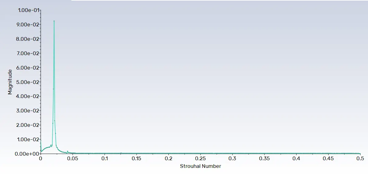
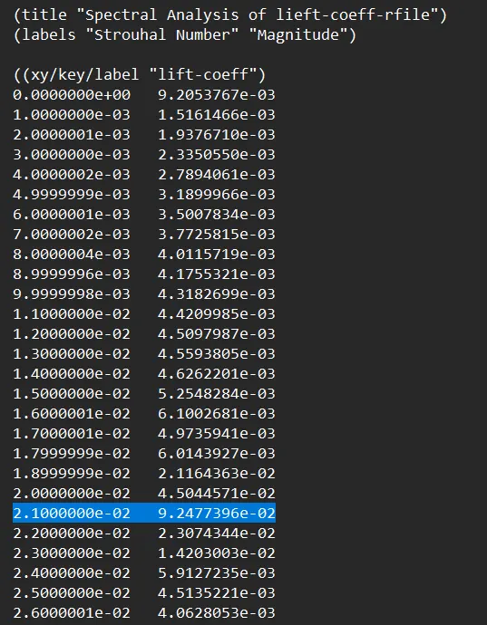
From the above plot of Strouhals Number and ,using highest value of magnitude Strouhal number was found to be 0.021.

---------------------------------------------------------------------------------------------------------------------------------------

PART-II

BC:

• Re = 10--->0.1 m/s
• Re = 100--->1 m/s
• Re = 1000--->10 m/s
• Re = 10000--->100 m/s
• Re = 100000--->1000 m/s

1)For Re = 10

Inlet velocity(U) -

Re = UL/nu

U = Re*(mu/rho)/L

In our case,diameter of the cylinder is 2 m ,therefore our characteristics length will be 2 m.

U = 10*(0.02/1)/2

U = 0.1 m/s

Residuals:

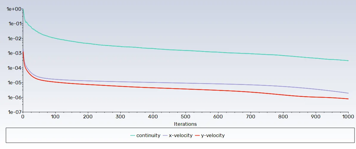
The flow has converged.

Vertex Average of Velocity:

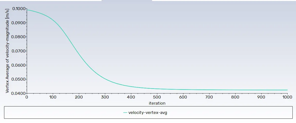
As the flow has very low velocity there is no fluctuations seen in the flow velocity at the designed vertex.

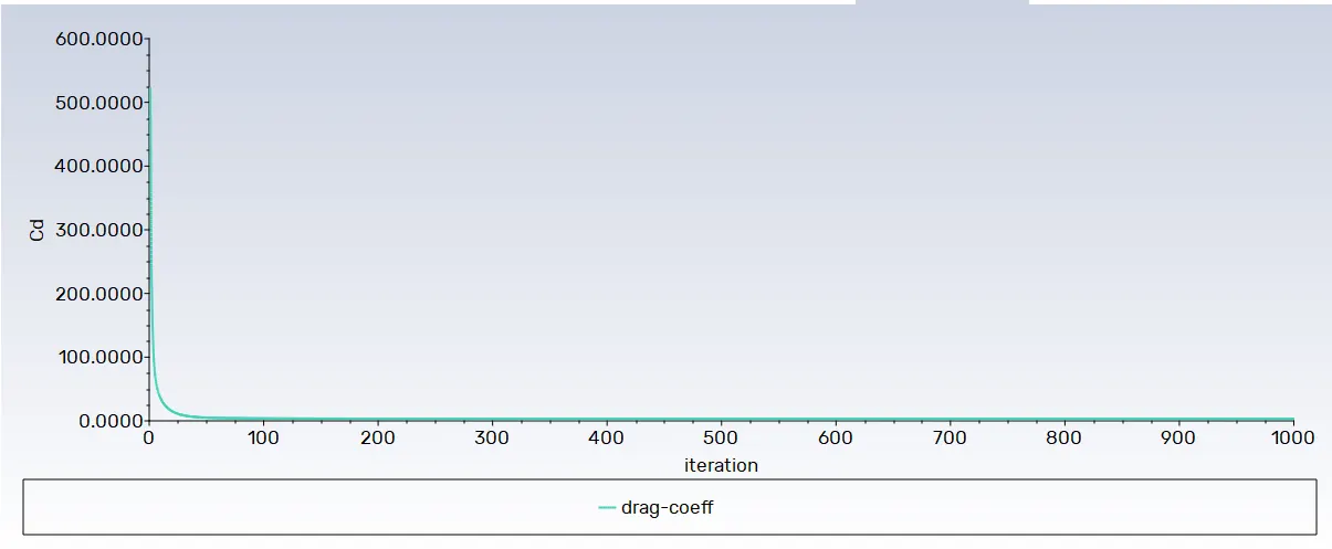
Coefficient of Drag:

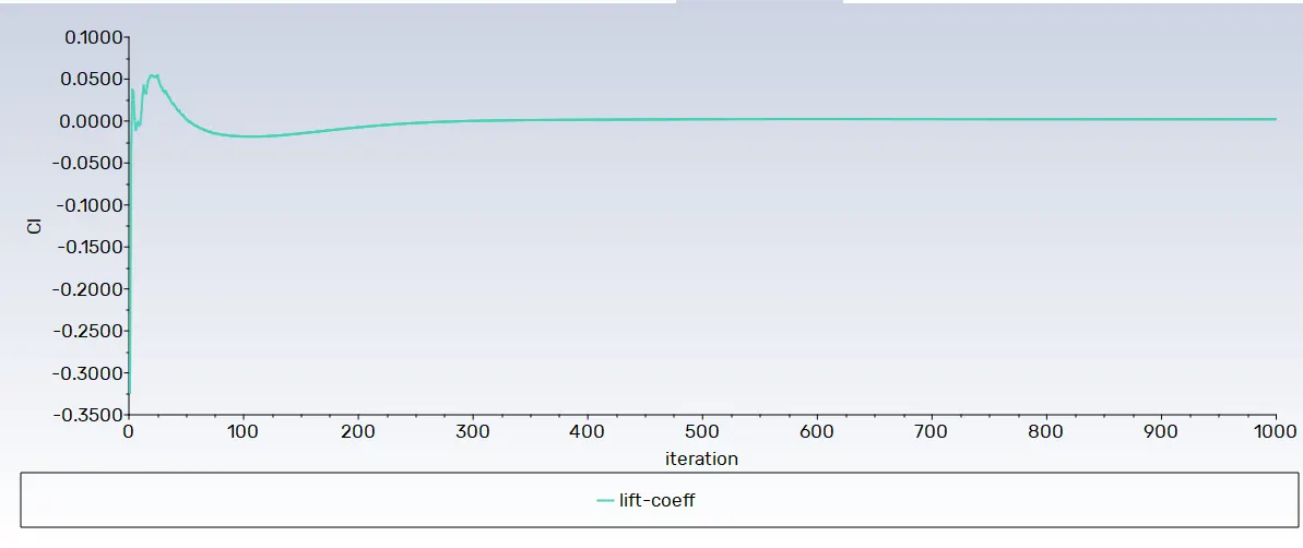
Coefficient of Lift:

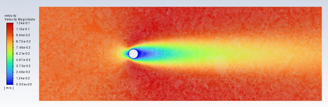
Velocity Contours:

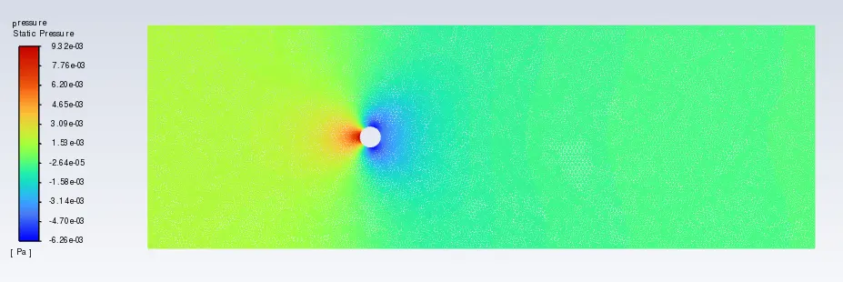
Pressure Contours:

Drag Coefficient = 3.3242244

Lift Coefficient = 0.00223

Average velocity at vertex = 0.0424 [m/s]

In scenarios of extremely slow flow, where viscosity is neglected, there is no flow separation or wake downstream of the cylinder. The flow remains symmetric from upstream to downstream, resulting in the absence of drag on the cylinder. However, it's important to note that this idealized flow condition is not representative of natural flows, where there is always some small amount of viscosity present in the fluid.

2)For Re = 100

Inlet velocity(U) -

Re = UL/nu

U = Re*(mu/rho)/L

U = 100*(0.02/1)/2

U = 1 m/s

Residuals:

All the residuals falls below 1e-4 thus we can say our flow has converged.

Vertex Average of Velocity:

Coefficient of Drag:

Coefficient of Lift:

Velocity Contours:

Pressure Contours:

Drag Coefficient = 1.3371

Lift Coefficient = 0.01124

Average velocity at vertex =0.63022[m/s]

As the flow velocity increases,the down stream vortices becomes unstable,separate from the body and are alternatively shed from the downstream.The wake is wide and generate large amount of drag.

3)For Re = 1000

Inlet velocity(U) -

Re = UL/nu

U = Re*(mu/rho)/L

U = 1000*(0.02/1)/2

U = 10 m/s

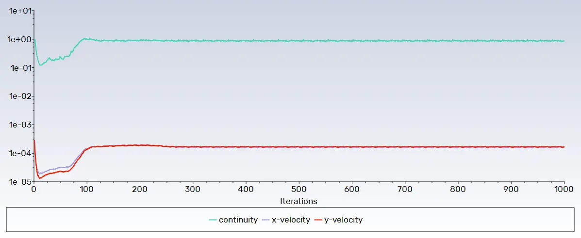
Residuals:

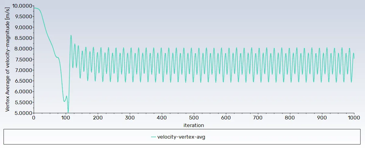
Vertex Average of Velocity:

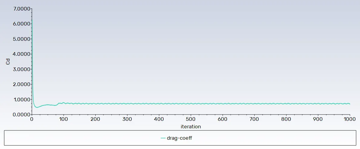
Coefficient of Drag:

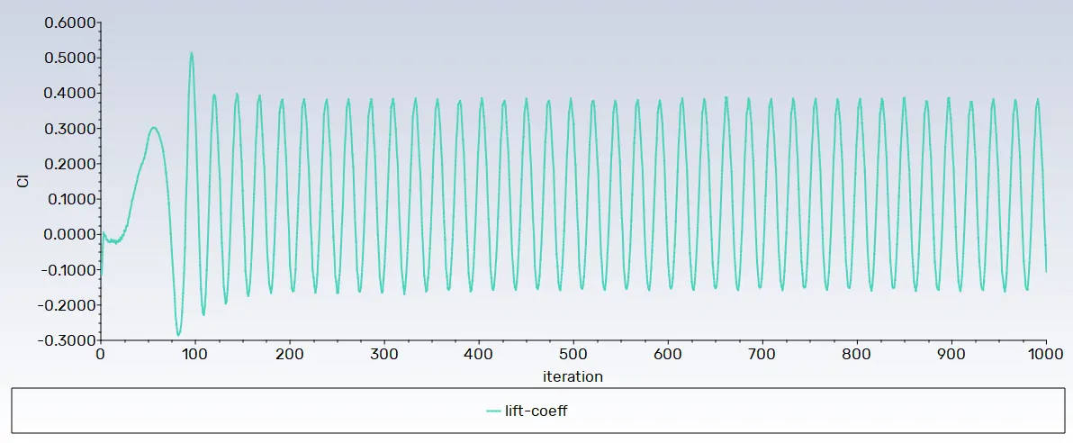
Coefficient of Lift:

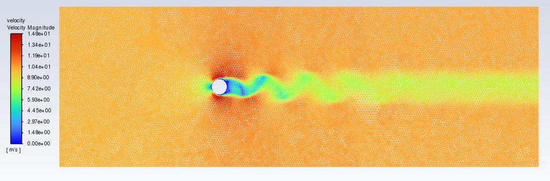
Velocity Contours:

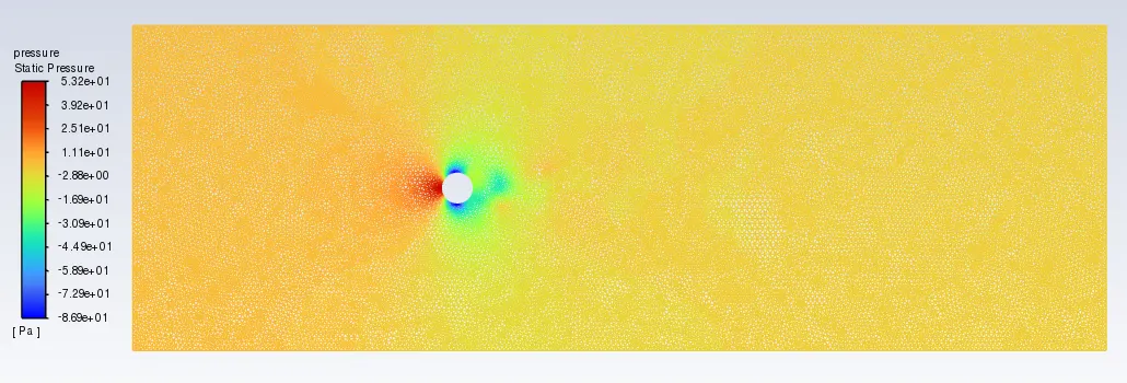
Pressure Contours:

Drag Coefficient = 0.7131

Lift Coefficient = 0.11405

Average velocity at vertex =7.2287[m/s]

With an increase in flow velocity, the downstream vortices lose stability, detach from the body faster, and are periodically shed downstream. This results in a wide wake and the generation of a substantial amount of drag contribute to a significant drag force on the cylinder.

4)For Re = 10000

Inlet velocity(U) -

Re = UL/nu

U = Re*(mu/rho)/L

U = 10000*(0.02/1)/2

U = 100 m/s

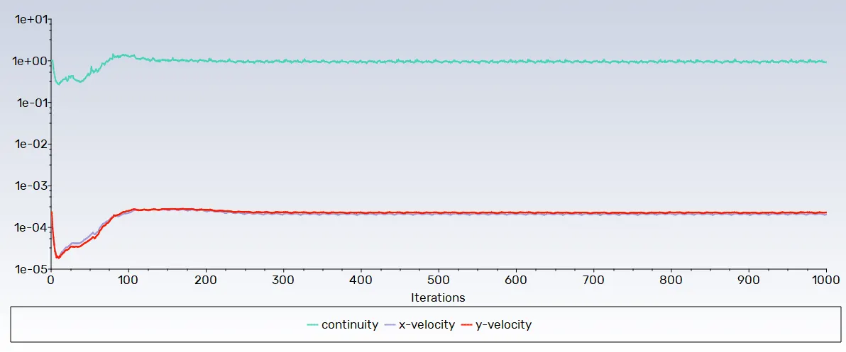
Residuals:

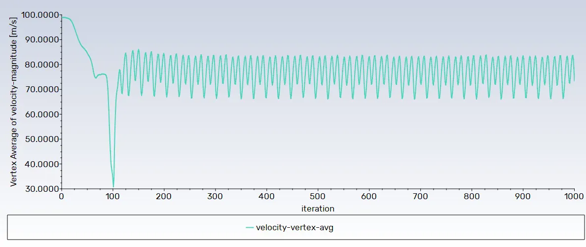
Vertex Average of Velocity:

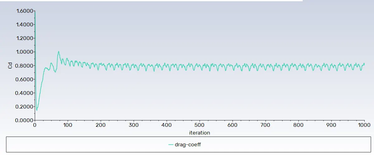
Coefficient of Drag:

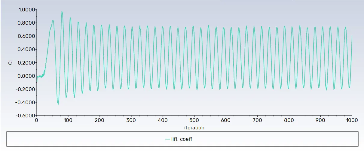
Coefficient of Lift:

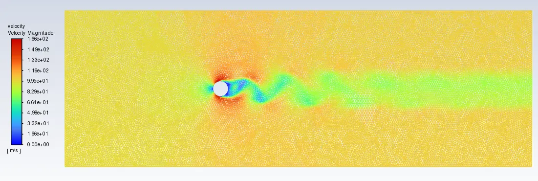
Velocity Contours:

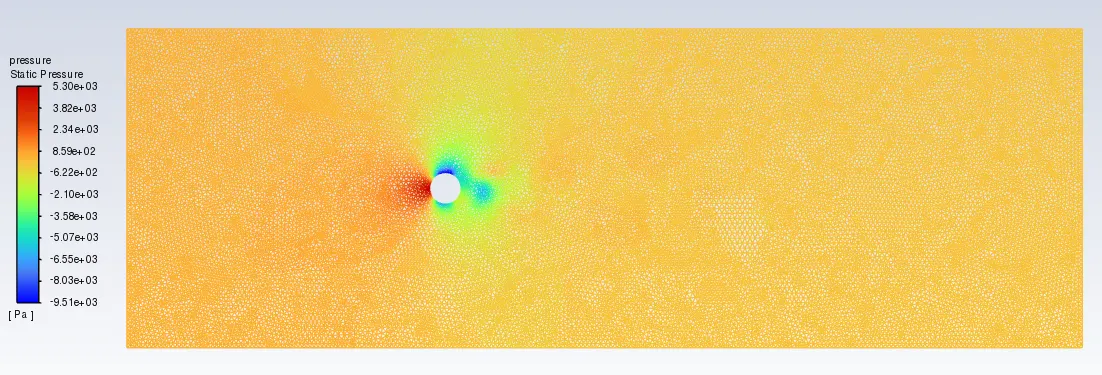
Pressure Contours:

Drag Coefficient = 0.7802

Lift Coefficient = 0.27685

Average velocity at vertex =74.9634 [m/s]

Further increase in flow velocity leads to the breakdown of periodic flow into a chaotic wake. While the flow remains laminar and orderly on the front side of the cylinder, the back side experiences chaotic wake formation, resulting in increased drag.

5)For Re = 100000

Inlet velocity(U) -

Re = UL/nu

U = Re*(mu/rho)/L

U = 100000*(0.02/1)/2

U = 1000 m/s

Residuals:

Vertex Average of Velocity:

Coefficient of Drag:

Coefficient of Lift:

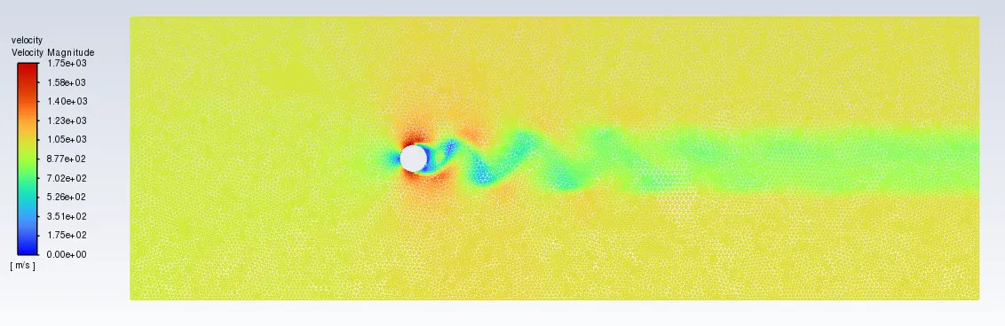
Velocity Contours:

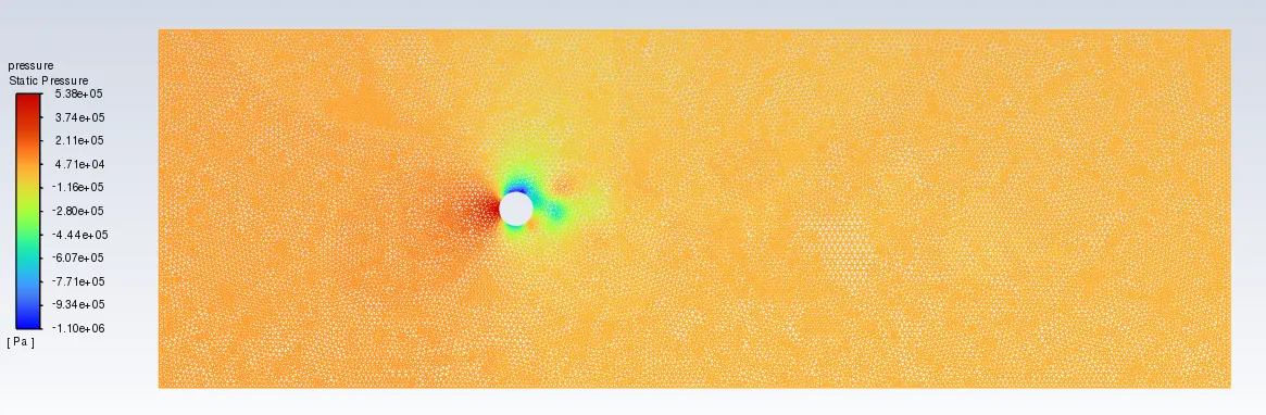
Pressure Contours:

Drag Coefficient =0.87615

Lift Coefficient = 0.2437

Average velocity at vertex = 756.3516 [m/s]

The boundary layer transitions into turbulent flow, leading to the shedding of vortices of varying scales in the wake region.

---------------------------------------------------------------------------------------------------------------------------------------

Flow Regimes and Cd Trends:

• Laminar Flow (Re = 10): At this low Re, the flow is smooth and predictable with a high Cd, typically higher, due to dominant viscous friction.
• Transitional Flow (Re = 100 - 1000): Flow starts transitioning from laminar to turbulent, causing fluctuations in Cd. There might be a slight decrease in Cd from the laminar value.
• Early Turbulent Flow (Re = 1000 - 10,000): Cd initially decreases due to delayed boundary layer separation and reduced pressure drag. However, skin friction drag increases, counteracting this reduction. The minimum Cd might be reached around Re =`3 x 10^5`.
• Developed Turbulent Flow (Re = 10,000 - 100,000): Cd usually stabilizes or slightly increases from its minimum value due to the dominant impact of skin friction drag at higher Re.

---------------------------------------------------------------------------------------------------------------------------------------

Examining the impact of the Reynolds number on the coefficient of drag and ensuring that the results are corroborated with established literature and maintaining an acceptable error margin within 5%.

Compilation of Cd, Cl and average velocity at vertex values corresponding to various Reynolds numbers obtained during steady-state and unsteady simulations:

Case (Re)	Drag Coefficient	Lift Coefficient	Average velocity at vertex (m/s)
Steady State
10	3.324	0.00223	0.0424
100	1.3371	0.01124	0.6302
1000	0.7131	0.11405	7.2287
10000	0.7829	0.27685	74.9634
100000	0.87615	0.2437	756.3516
Unsteady state
Re=100	1.341	0.0166	0.6861

Reference Table [1] depicting Cd values associated with specific Reynolds numbers.

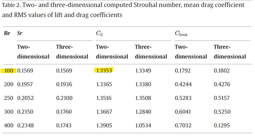
Comparing above results for Re with literature [1] - in Literature for Re = 100 cofficient of drag is 1.3353 and from simulation the obtained drag cofficient for Re = 100 is 1.3371318 (steady-state) & 1.341 (Transient-state).

Thus, there is error of less than 5% in between the literature and simulation values.

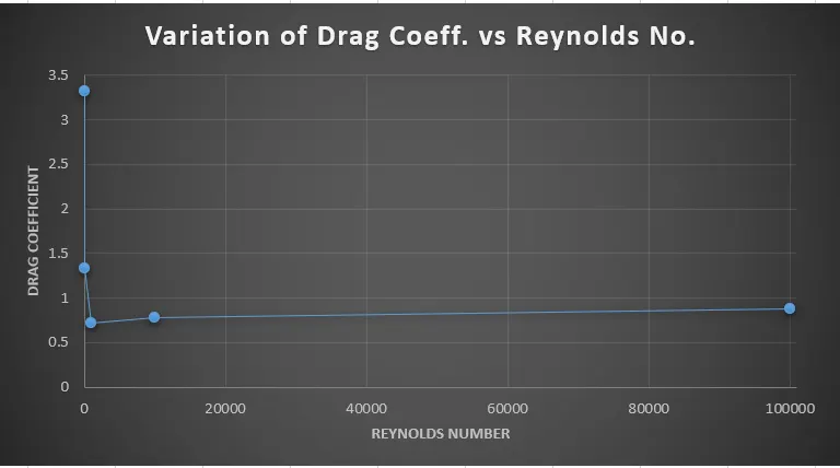
The above graph shows how drag Cofficient is decreases as the Reynolds no. increases and after Re= 1000, the change in drag coefficient value is very less.

Conclusion:

• The steady-state solver captures a stabilized flow by neglecting time.The unsteady-state solver initiates recording from t = 0, providing dynamic insights into the flow evolution.
• No vortex shedding is observed at Re = 10. Vortex shedding becomes pronounced at Re = 1000, minimal at Re = 10,000, and forms a small street at Re = 100,000.
• Reynolds Number Effects on Coefficients:Drag decreases while lift increases with higher Reynolds numbers. At Re = 10,000, a slight increase in drag is observed, and at Re = 100,000, a slight decrease in lift occurs.
• Developed Turbulent Flow (Re = 10,000 - 100,000): Cd usually stabilizes or slightly increases from its minimum value due to the dominant impact of skin friction drag at higher Re.
• Increased velocity raises turbulent drag beyond laminar values.
• During the laminar to turbulent transition, turbulent drag can be lower than laminar drag in a specific Reynolds range.
• Both steady and transient simulations exhibit vortex shedding.
• Transient simulations provide more realistic results regarding vortex shedding dynamics.
• Calculating the Strouhal Number is feasible only in transient simulations due to the frequency variation with time.

References:

1. Wikipedia

2. Fluid Mechanics Textbok -Cengel

3.Reference Research Paper:- https://www.sciencedirect.com/science/article/pii/S0307904X08000243