Week 7 - Simulation of a 1D Super-sonic nozzle flow simulation using Macormack Method
1) Non- conservative form
Please find the code for non-conservative form
clear all
close all
clc

%input
n=31;
x=linspace(0,3,n);
dx= x(2)-x(1);
gama=1.4    ;

%calculating initial proffile

rho= 1-0.3146*(x);
t = 1-0.2314*x; % t=temprature
v=(0.1+1.09*x).*t.^0.5;
%area
a= 1+2.2*(x-1.5).^2;

%time step

nt=1000;
dt=0.04;
th=round(n/2);

cfl=max((v+sqrt(t))*dt/dx);

%outer loop

for k=1:nt

    %making a copy
    rho_old=rho;
    v_old=v;
    t_old=t;


    %predicted step
    for j=2:n-1

        dvdx= (v(j+1)-v(j))/dx;
        drhodx=(rho(j+1)-rho(j))/dx;
        dtdx=(t(j+1)-t(j))/dx;
        dlogadx=(log(a(j+1))-log(a(j)))/dx;

        %continuity equation
        drhodt_p(j)=-rho(j)*dvdx-rho(j)*v(j)*dlogadx-v(j)*drhodx;

        %momentum  equation

        dvdt_p(j) =-v(j)*dvdx-(1/gama)*(dtdx+(t(j)/rho(j)))*drhodx;

        %energy equation
        dtdt_p(j) =-v(j)*dtdx-(gama-1)*t(j)*(dvdx+v(j)*dlogadx);

        %solution update

        rho(j)= rho(j)+drhodt_p(j)*dt;
        v(j)=v(j)+dvdt_p(j)*dt;
        t(j)=t(j)+dtdt_p(j)*dt;
    end
    %corector method
    for j=2:n-1

        dvdx= (v(j)-v(j-1))/dx;
        drhodx=(rho(j)-rho(j-1))/dx;
        dtdx=(t(j)-t(j-1))/dx;
        dlogadx=(log(a(j))-log(a(j-1)))/dx;

        %continuity equation
        drhodt_c(j) =-rho(j)*dvdx-rho(j)*v(j)*dlogadx-v(j)*drhodx;

        %momentum  equation

        dvdt_c(j) =-v(j)*dvdx-(1/gama)*(dtdx+(t(j)/rho(j)))*drhodx;

        %energy equation
        dtdt_c(j) =-v(j)*dtdx-(gama-1)*t(j)*(dvdx+v(j)*dlogadx);


    end

    %computing the avg.

    dvdt= 0.5*(dvdt_p+dvdt_c);
    drhodt= 0.5*(drhodt_p+drhodt_c);
    dtdt=0.5*(dtdt_p+dtdt_c);

    %final solution
    for i = 2:n-1
        rho(i)=rho_old(i)+drhodt(i)*dt;
        v(i)= v_old(i) + dvdt(i)*dt;
        t(i)= t_old(i)+dtdt(i)*dt;

    end
    %apply BC
    %inlet BC
    v(1)=2*v(2)-v(3);


    %outlet
    v(n)=2*v(n-1)-v(n-2);
    rho(n)=2*rho(n-1)-rho(n-2);
    t(n)=2*t(n-1)-t(n-2);


    %pressure
    p=rho.*t;

    %mac no.
    M=v./sqrt(t);
    %mass flow rate
    m=rho.*a.*v;


    figure(3)
    if k==1
        plot(x,m)
    end
    hold on
    if k==50
        plot(x,m)
    end
    if k==250
        plot(x,m)
    end
    if k==500
        plot(x,m)
    end
    if k==750
        plot(x,m)
    end
    if k==1000
        plot(x,m)
    end

    rho_th(k) =rho(th);
    v_th(k) =v(th);
    t_th(k) =t(th);
    p_th(k) =p(th);
    M_th(k) =M(th);
end
xlabel('nozzle length')
ylabel('mass flow rate')
legend('1dt','50dt','250dt','500dt','750dt','1000dt')
title('steady state mass flow rate profile at diff. time step')


figure(1)
subplot(5,1,1)
plot(x,v)
xlabel('nozzle length')
ylabel('velovity')
title(sprintf('time step=%d',k))
pause(0.03)

subplot(5,1,2)
plot(x,t)
xlabel('nozzle length')
ylabel('temprature')
title(sprintf('time step=%d',k))
pause(0.03)

subplot(5,1,3)
plot(x,rho)
xlabel('nozzle length')
ylabel('density')
title(sprintf('time step=%d',k))
pause(0.03)


subplot(5,1,4)
plot(x,M)
xlabel('nozzle length')
ylabel('Mac no')
title(sprintf('time step=%d',k))
pause(0.03)


subplot(5,1,5)
plot(x,p)
xlabel('nozzle length')
ylabel('pressure')
title(sprintf('time step=%d',k))
pause(0.03)

figure(2)

plot(x,m)
xlabel('nozzle length')
ylabel('mass flow rate')
title('steady state mass flow rate profile')
pause(0.03)


%ploting throt value

figure(4)
subplot(5,1,1)
plot(v_th)
xlabel('time step')
ylabel('velovity')
title(sprintf('time step=%d',k))
pause(0.03)

subplot(5,1,2)
plot(t_th)
xlabel('time step')
ylabel('temprature')
title(sprintf('time step=%d',k))
pause(0.03)

subplot(5,1,3)
plot(rho_th)
xlabel('time step')
ylabel('density')
title(sprintf('time step=%d',k))
pause(0.03)


subplot(5,1,4)
plot(M_th)
xlabel('time step')
ylabel('Mac no')
title(sprintf('time step=%d',k))
pause(0.03)


subplot(5,1,5)
plot(p_th)
xlabel('time step')
ylabel('pressure')
title(sprintf('time step=%d',k))
pause(0.03)
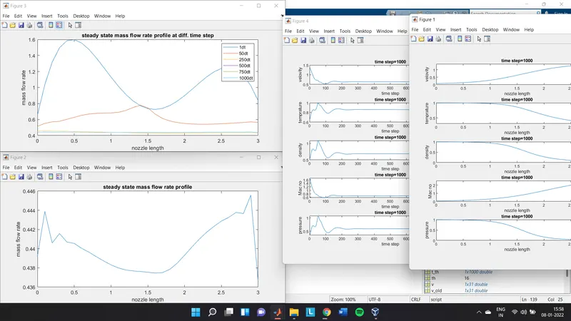
The two graphs fig(1) and fig(2) shows the mass flow rate movement
on fig. 1 it is different form in diff. time steps
as time step increases the flow is converged so a steady straight line can be ssen as time step increases
in fig. 2 the mass flow rate along with the nozzle length i.e. the rate of flow along the length, as it is a supersonic nozzle the flow in right is more and as a in throt area it is lowest
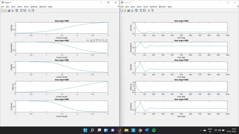
these two graphs are very important, in first one the graph shows how the diff. quantities changes along with the flow in nozzle
as we can see the pressure drops, the density drops and velocity increases, all this can state that it’s a supersonic outlet
in 2 fig. it shows how the problem is converged as the values at throt are calculated with time loop, the starting disturbance are the loop we take to converge the actual solution an as the values get closer in it shown that values are converge and a specific value can be stated as the quantity at throt
2) conservative form
clear all
close all
clc

%input
n=31;
x=linspace(0,3,n);
dx= x(2)-x(1);
gama=1.4    ;

%calculating initial proffile


for i=1:n

    if x(i)<=0.5
        rho(i) = 1;
        t(i) = 1;
    end
    if x(i)>0.5 && x(i)<=1.5
        rho(i) = 1-0.366*(x(i)-0.5);
        t(i) = 1-0.167*(x(i)-0.5);
    end

    if x(i)>1.5
        rho(i) = 0.634-0.3879*(x(i)-1.5);
        t(i) = 0.833-0.3507*(x(i)-1.5);
    end


end

%area
a= 1+2.2.*(x-1.5).^2;
v=0.59./(rho.*a);
u1=rho.*a;
u2= rho.*a.*v;
u3=u1.*(t/(gama-1)+(gama/2)*v.^2);

nt=1400;
dt=0.0267;
gama=1.4;
th=round(n/2);

%cfl=max((v+sqrt(t))*dt/dx);


%outer loop

for k=1:nt

    %making a copy
    u1_old=u1;
    u2_old=u2;
    u3_old=u3;

    f1=u2;
    f2=u2.^2./u1 + ((gama-1)/gama)*(u3-(gama/2)*(u2.^2./u1));
    f3 = (gama*u2.*u3./u1)-0.5*gama*(gama-1)*(u2.^3./u1.^2);


    %predicted step
    for j=2:n-1


        %continuity equation
        du1dt_p(j)=-(f1(j+1)-f1(j))/dx;

        j2= (1/gama)*rho(j)*t(j)*(a(j+1)-a(j))/dx;
        %momentum  equation

        du2dt_p(j) =-(f2(j+1)-f2(j))/dx+j2;

        %energy equation
        du3dt_p(j) =-(f3(j+1)-f3(j))/dx;

        %solution update

        u1(j)= u1(j)+du1dt_p(j)*dt;
        u2(j)=u2(j)+du2dt_p(j)*dt;
        u3(j)=u3(j)+du3dt_p(j)*dt;
    end

    %predictor updte

    rho=u1./a;
    t=(gama-1)*((u3./u1)-(gama/2)*(u2./u1).^2);
    v = u2./u1;
    f1=u2;
    f2=u2.^2./u1 + ((gama-1)/gama)*(u3-(gama/2)*(u2.^2./u1));
    f3 = (gama*u2.*u3./u1)-0.5*gama*(gama-1)*(u2.^3./u1.^2);


    %corector method
    for j=2:n-1


        %continuity equation
        du1dt_c(j)=-(f1(j)-f1(j-1))/dx;

        j2= (1/gama)*rho(j)*t(j)*(a(j)-a(j-1))/dx;
        %momentum  equation

        du2dt_c(j) =-(f2(j)-f2(j-1))/dx+j2;

        %energy equation
        du3dt_c(j) =-(f3(j)-f3(j-1))/dx;

    end

    %computing the avg.
    du1dt=0.5*(du1dt_p+du1dt_c);
    du2dt=0.5*(du2dt_p+du2dt_c);
    du3dt=0.5*(du3dt_p+du3dt_c);

    %final solution
    for p = 2:n-1
        u1(p)= u1_old(p)+du1dt(p)*dt;
        u2(p)= u2_old(p)+du2dt(p)*dt;
        u3(p)= u3_old(p)+du3dt(p)*dt;

  end
      %final update
    rho=u1./a;
    t=(gama-1)*(u3./u1-(gama/2)*(u2./u1).^2);
    v= u2./u1;

    % apply BC
    %inlet BC
    u1(1)=a(1);
    u2(1)=2*u2(2)-u2(3);
    v(1) = u2(1)/u1(1);
   %u3(1)=u1(1)*(t(1)/(gama-1))+0.5*gama*v(1)^2; ERROR (Brackets)
    u3(1)=u1(1)*(t(1)/(gama-1)+0.5*gama*v(1)^2);


    %outlet
    u1(n)=2*u1(n-1)-u1(n-2);
    u2(n)=2*u2(n-1)-u2(n-2);
    u3(n)=2*u3(n-1)-u3(n-2);

    %pressure
    p=rho.*t;

    %mac no.
    M=v./sqrt(t);
    %mass flow rate
    m=rho.*a.*v;


    figure(1)
    if k==1
        plot(x,m)
    end
    hold on
    if k==50
        plot(x,m)
    end
    if k==250
        plot(x,m)
    end
    if k==500
        plot(x,m)
    end
    if k==750
        plot(x,m)
    end
    if k==1000
        plot(x,m)
    end

    rho_th(k) =rho(th);
    v_th(k) =v(th);
    t_th(k) =t(th);
    p_th(k) =p(th);
    M_th(k) =M(th);
end
xlabel('nozzle length')
ylabel('mass flow rate')
legend('1dt','50dt','250dt','500dt','750dt','1000dt')
title('steady state mass flow rate profile at diff. time step')
hold off

figure(2)
subplot(5,1,1)
plot(x,v)
xlabel('nozzle length')
ylabel('velovity')
title(sprintf('time step=%d',k))

subplot(5,1,2)
plot(x,t)
xlabel('nozzle length')
ylabel('temprature')
title(sprintf('time step=%d',k))


subplot(5,1,3)
plot(x,rho)
xlabel('nozzle length')
ylabel('density')
title(sprintf('time step=%d',k))


subplot(5,1,4)
plot(x,M)
xlabel('nozzle length')
ylabel('Mac no')
title(sprintf('time step=%d',k))


subplot(5,1,5)
plot(x,p)
xlabel('nozzle length')
ylabel('pressure')
title(sprintf('time step=%d',k))

figure(3)

plot(x,m)
xlabel('nozzle length')
ylabel('mass flow rate')
title('steady state mass flow rate profile')


%ploting throt value

figure(4)
subplot(5,1,1)
plot(v_th)
xlabel('time step')
ylabel('velovity')
title(sprintf('time step=%d',k))

subplot(5,1,2)
plot(t_th)
xlabel('time step')
ylabel('temprature')
title(sprintf('time step=%d',k))

subplot(5,1,3)
plot(rho_th)
xlabel('time step')
ylabel('density')
title(sprintf('time step=%d',k))


subplot(5,1,4)
plot(M_th)
xlabel('time step')
ylabel('Mac no')
title(sprintf('time step=%d',k))


subplot(5,1,5)
plot(p_th)
xlabel('time step')
ylabel('pressure')
title(sprintf('time step=%d',k))
if we see there isnt any major diff. between conservative and non-conservative form solution wise only for CFD anlysus they differ
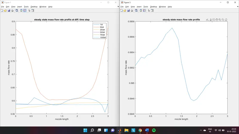
In fig 1 the different mass flow rate on different time step is shown
and steady state mass flow rate is shown in fig 2
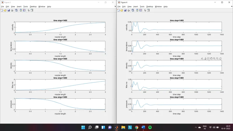
In above fig. fig. 1 shows the variation of quantities along the nozzle length, as it a supersonic outlet as similar to non-conservative flow the pressure drops the density drops and the velocity increases,
in fig. 2 the quantities are converged along with time and the become stable as the flow continues