Week 5.1 - Mid term project - Solving the steady and unsteady 2D heat conduction problem
clear all
close all
clc

% steady state heat conducrion equation d^2t/dx^2 + d^2t/dy^2=0

nx=10;
ny=10;

T=450*ones(nx,ny);


%k1=aplha*(dt/dx^2)
%fase tempreture
TL= 400;
TR= 800;
TT = 600;
TB= 900;

%BC
T(:,1)=TL;
T(:,ny)=TR;
T(1,:)=TT;
T(nx,:)=TB;
%edge refinement
T(1,1)=(T(2,1)+T(1,2))/2;
T(nx,1)=(T(nx-1,1)+T(nx,2))/2;
T(nx,ny)= (T(nx-1,ny)+T(nx,ny-1))/2;
T(1,ny)=(T(2,ny)+T(1,ny-1))/2;

Told=T;
Tinitial = T;

% iteration process 1. jacobi 2. gs 3. sor
% 1) jacobi method

error = 9e9;
tol = 1e-4;
jac_itel=0

while(error>tol)

    for i=2:nx-1
        for j= 2:ny-1

            T(i,j)= 0.25*(T(i+1,j) + Told(i-1,j)+Told(i,j-1)+Told(i,j+1));
        end
    end

    error= max(max(abs(T-Told)));
    Told=T;
    jac_itel=jac_itel+1;
    figure(1)
    contourf(flipud(T),'ShowText','ON')

    title(sprintf('steady state jacobi iteration=%d',jac_itel))
    pause(0.003)


end

colorbar

% reinitializing
T=Tinitial;
Told=T;
error=9e9;
gs_iter=0;
% GS method for itteration

while(error>tol)

    for i=2:nx-1
        for j= 2:ny-1

            T(i,j)= 0.25*(T(i+1,j) + T(i-1,j)+T(i,j-1)+Told(i,j+1));
        end
    end

    error= max(max(abs(T-Told)));
    Told=T;
    gs_iter=gs_iter+1;
    figure(2)
    contourf(flipud(T),'ShowText','ON')

    title(sprintf('steady state GS iteration=%d',gs_iter))
    pause(0.003)


end
colorbar
%reinitialise for SOR
T=Tinitial;
Told=T;
error=9e9;

%SOR iteration

SOR_iter=0;
omega=1.5;

while(error>tol)

    for i=2:nx-1
        for j= 2:ny-1

            TGS(i,j)= 0.25*(T(i+1,j) + T(i-1,j)+T(i,j-1)+Told(i,j+1));
            T(i,j)=(1-omega)*Told(i,j) + omega*TGS(i,j);


        end
    end

    error= max(max(abs(T-Told)));
    Told=T;
    SOR_iter=SOR_iter+1;
    figure(3)
    contourf(flipud(T),'ShowText','ON')

    title(sprintf('steady state SOR iteration=%d',SOR_iter))
    pause(0.003)


end
colorbar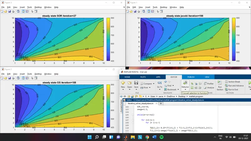
1) Steady state iteration count
Above graph is for steady 2D state calculation of heat conduction equation,
from all graph being same, we can understand the ans. by all 3 methods are same at the end only the no. of iterations it requires varies like in Jacobi method the iteration value is highest, and accordingly SOR method has least iteration.
so, the SOR method is faster than compare to other two
2) Implicit calculation
please find code and graph screen shots below
clear all
close all
clc

% steady state heat conducrion equation d^2t/dx^2 + d^2t/dy^2=0

nx=10;
ny=10;

T=450*ones(nx,ny);


%k1=aplha*(dt/dx^2)
%fase tempreture
TL= 400;
TR= 800;
TT = 600;
TB= 900;

%BC
T(:,1)=TL;
T(:,ny)=TR;
T(1,:)=TT;
T(nx,:)=TB;
%edge refinement
T(1,1)=(T(2,1)+T(1,2))/2;
T(nx,1)=(T(nx-1,1)+T(nx,2))/2;
T(nx,ny)= (T(nx-1,ny)+T(nx,ny-1))/2;
T(1,ny)=(T(2,ny)+T(1,ny-1))/2;

Told=T;
Tinitial = T;
Tprev=T;
%timestep
dt=1e-2;
%grid spacing
dx=1e-2;
dy=1e-2;
%thermal diffusity
alpha = 0.015;

k1=alpha*(dt/dx^2);
k2=alpha*(dt/dy^2);

% iteration process 1. jacobi 2. gs 3. sor
% 1) jacobi method

error = 9e9;
conv=9e9;
tol = 1e-4;
jac_itel=0;
Jac_time_iter=0;

%time loop
while(conv>tol)
    %space loop
    while(error>tol)

        for i=2:nx-1
            for j= 2:ny-1

                T(i,j)= (1+2*k1+2*k2)^-1*(Tprev(i,j)+ k1*(Told(i-1,j)+Told(i+1,j))+k2*(Told(i,j-1)+Told(i,j+1)));
            end
        end

        error= max(max(abs(T-Told)));
        Told=T;
        jac_itel=jac_itel+1;
        figure(1)
        contourf(flipud(T),'ShowText','ON')

        title(sprintf('Transient imlicit jacobi iteration=%d \nTime iterations=%d',jac_itel,Jac_time_iter))
        pause(0.003)

    end
    conv= max(max(abs(T-Tprev)));
    Tprev=T;
    Jac_time_iter=Jac_time_iter+1;
    error=9e9;


end


colorbar

% reinitializing
T=Tinitial;
Told=T;
error=9e9;
gs_iter=0;
gs_time=0;
conv=9e9;
Tprev=T;
% GS method for itteration

%time loop
while(conv>tol)
    %space loop
    while(error>tol)

        for i=2:nx-1
            for j= 2:ny-1

                T(i,j)= (1+2*k1+2*k2)^-1*(Tprev(i,j)+ k1*(T(i-1,j)+Told(i+1,j))+k2*(T(i,j-1)+Told(i,j+1)));
            end
        end

        error= max(max(abs(T-Told)));
        Told=T;
        gs_iter=gs_iter+1;
        figure(2)
        contourf(flipud(T),'ShowText','ON')

        title(sprintf('Transient imlicit gs iteration=%d \nTime iterations=%d',gs_iter,gs_time))
        pause(0.003)

    end
    conv= max(max(abs(T-Tprev)));
    Tprev=T;
    gs_time=gs_time+1;
    error=9e9;


end
colorbar

%reinitialise for SOR
T=Tinitial;
Told=T;
error=9e9;
Tprev=T;
conv=9e9;


%SOR iteration

SOR_iter=0;
SOR_time_iter=0;
omega=1.5;

%time loop
while(conv>tol)
    %space loop
    while(error>tol)

        for i=2:nx-1
            for j= 2:ny-1

                TGS(i,j)= (1+2*k1+2*k2)^-1*(Tprev(i,j)+ k1*(T(i-1,j)+Told(i+1,j))+k2*(T(i,j-1)+Told(i,j+1)));
                T(i,j) = (1-omega)*Told(i,j)+omega*(TGS(i,j));
            end
        end

        error= max(max(abs(T-Told)));
        Told=T;
        SOR_iter=SOR_iter+1;
        figure(3)
        contourf(flipud(T),'ShowText','ON')

        title(sprintf('Transient imlicit SOR iteration=%d \nTime iterations=%d',SOR_iter,SOR_time_iter))
        pause(0.003)

    end
    conv= max(max(abs(T-Tprev)));
    Tprev=T;
    SOR_time_iter=SOR_time_iter+1;
    error=9e9;


end
colorbar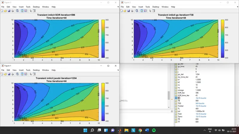
In implicit method the calculation goes step by step approaching through time and gradients
Well, the end output is same as steady state but the in between flow or the process which the changes go through are clearer in this way.
3) explicit method for time iteration
please find the code and graph PS
clear all
close all
clc

% steady state heat conducrion equation d^2t/dx^2 + d^2t/dy^2=0

nx=10;
ny=10;

T=450*ones(nx,ny);


%k1=aplha*(dt/dx^2)
%fase tempreture
TL= 400;
TR= 800;
TT = 600;
TB= 900;

%BC
T(:,1)=TL;
T(:,ny)=TR;
T(1,:)=TT;
T(nx,:)=TB;
%edge refinement
T(1,1)=(T(2,1)+T(1,2))/2;
T(nx,1)=(T(nx-1,1)+T(nx,2))/2;
T(nx,ny)= (T(nx-1,ny)+T(nx,ny-1))/2;
T(1,ny)=(T(2,ny)+T(1,ny-1))/2;


Tprev=T;
%timestep
dt=1e-2;
%grid spacing
dx=5e-2;
dy=5e-2;
%thermal diffusity
alpha = 0.015;

k1=alpha*(dt/dx^2);
k2=alpha*(dt/dy^2);

% Time iterative solver


cfl=k1+k2;
conv=9e9;
tol = 1e-4;

time_iter=0;

%time loop
while(conv>tol)

    for i=2:nx-1
        for j= 2:ny-1

            T(i,j)= (1-2*k1-2*k2)*Tprev(i,j)+ k1*(Tprev(i-1,j)+Tprev(i+1,j))+k2*(Tprev(i,j-1)+Tprev(i,j+1));
        end
    end

    conv= max(max(abs(T-Tprev)));
    Tprev=T;
    time_iter=time_iter+1;

    figure(1)
    contourf(flipud(T),'ShowText','ON')

    title(sprintf('Transient explicit time iteration=%d',time_iter))
    pause(0.05)
end

colorbar
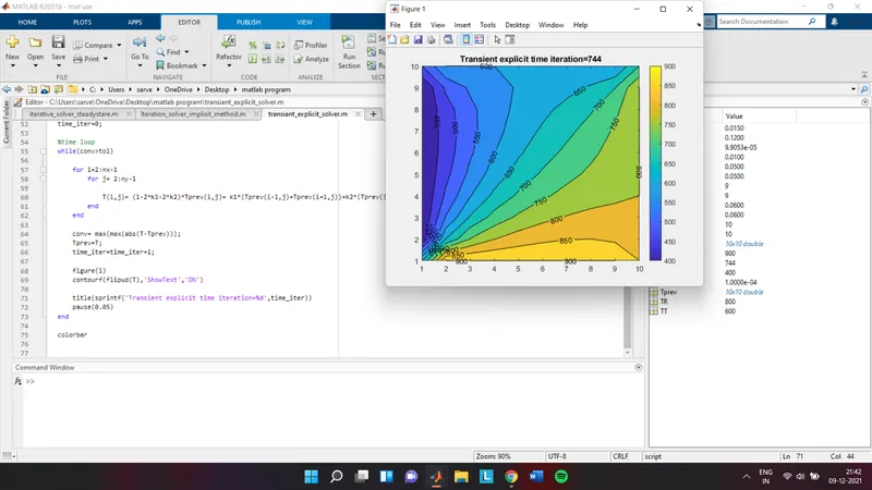
In explicit method only time loop is required, as all adjacent values we use to calculate the next value in next time step is taken from the previous matrix, or previous time step,
so, no need of space loop also in implicit method as we have to take values from two matrix the three diff. methods can be use but as in this method all values in RHS are know so no complex calculation, though the output is same, there are some advantages and disadvantages.
as in explicit we have to consider clf term which is k1+k2 which should not exceed 0.5 in 2D conduction, otherwise it can blow up the entire solution, so mostly there are some criteria which needs to be taken under consideration for choosing any of these methods