Week 5 - Rayleigh Taylor Instability

PROJECT REPORT

Aim:

• Perform Rayleigh-Taylor instability simulation in Ansys fluent, for two different mesh size with basic mesh size of 0.5mm and record the difference
• Also creating a user define fluid with high density and performing the same simulation to record the difference in instability

Theory:

The Rayleigh-Taylor instability occurs on the interface of two fluids which are immiscible, in which the fluid with more density rests on the light fluid occurs in instable mixing of both fluid which gives out a beautiful flow view which shows some mushroom like shape, while eventually the denser fluid is trying to get at the bottom

Types of models based on Rayleigh- Taylor instabilities:

There are several models, some of them are as follow

• Richtmyer – Meshkov instability:
• Richtmyer- meshkov instability occurs when two fluids of different density are impulsively accelerated. Normally this is by the passage of a shock wave. This is followed by a nonlinear regime with bubbles appearing in the case of light fluid penetrating in heavy fluid, in heavy fluid case spikes appears as it flows separating the light fluid
• This model is based on the Rayleigh- Taylor in stability calculation, it can also be considered as the impulsive acceleration limit of the Rayleigh – Taylor instability.
• Kelvin-Helmholtz instability
• In this type the both fluids are in motion, typically occurs when both fluid layers interact while flowing in opposite side, which cause in some initial instability in the interference
• This small instability starts to grow as there the starting in stability causes in pressure difference in the both layers, as a result it causes some repetitive shapes in the flow. Which can be seen in clouds, on the surface of Jupiter planet, and many such applications

SET UP:

• Geometry:

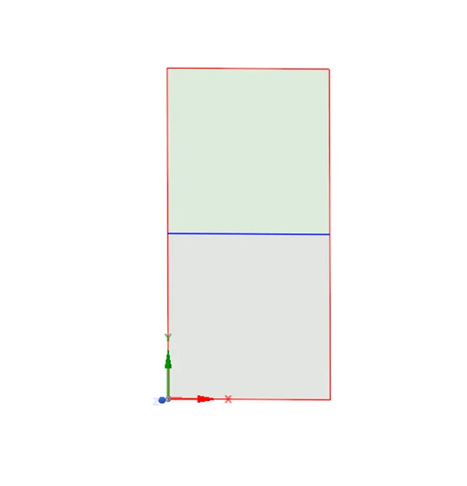
We start with two squares of 20 x 20mm dimension were created along the xy plane in two different components. Will convert it in plane by pull tool. Then use share tropology between both of them, and as our water is going to be on top and air at the bottom, we can name two squares accordingly.

MESH:

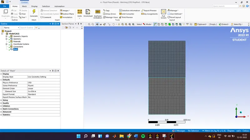
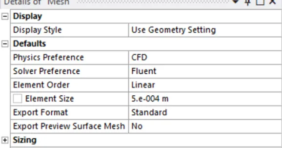
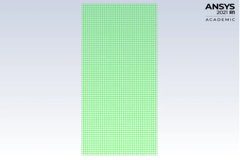
Mesh is simple a simple mesh is used as we have to use 0.5mm as base mesh so we have set 2 cases accordingly. In first case the mesh is of element size 0.5mm and in second case the mesh size is of 0.2mm

CASE I:

SET UP:

Mesh is setup and, in this case, we are going to use gravity so as our module is on xy plane the gravity should be in -Y direction

We are using transient time step and pressure base solver

As the velocity is going to be very low the flow is going to be laminar and we are using multifaced model to make interface of two different fluid our primary fluid is air and our secondary fluid is water. Water is located above the air to capture the instability it will go through to settle down at the bottom

We will run the solution for 1500 timestep with 0.005-time step size

SOLUTION:

Case I:

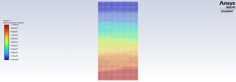
Mesh size of 0.5mm

RESULTS:

Steady form after the simulation

Link:

https://drive.google.com/drive/folders/11p___L_2Xnp-ACqPJ3wQIZB6lYTAnx2x?usp=sharing

Case 2:

Here the mesh size is finer with 0.1mm

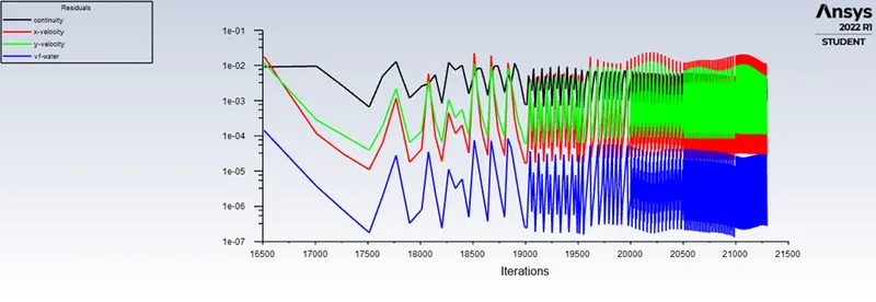
RESIDUALS:

RESULTS

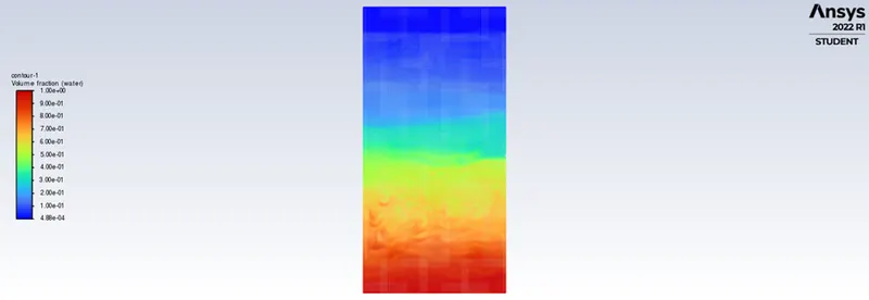
As we can see the image become sharper and more precise as we reduce the mesh size

LINK:

https://drive.google.com/drive/folders/11p___L_2Xnp-ACqPJ3wQIZB6lYTAnx2x?usp=sharing

CASE 3:

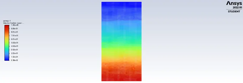
In this we are going to create a user define material and replace it with water and record the difference

With density = 400kg/m^3

Viscosity = 0.001 kg/m-s

RESULTS:

LINK:

https://drive.google.com/drive/folders/11p___L_2Xnp-ACqPJ3wQIZB6lYTAnx2x?usp=sharing

In this case it took less time to reach the steady state

ATWOOD NUMBER:

The Atwood number is a dimensionless number, used to study of hydrodynamic instabilities in density stratified flows. It is dimensionless density ratio defines as

A = `rho`1 - `rho`2 / `rho`1 +`rho`2

`rho`1 = Density of heavier fluid

`rho`2 = Density of lighter fluid

In case 1 and 2

`rho`1 = 1000

`rho`2 = 1.225

A = 1000-1.225/1000+1.225 = 0.9975

In case 3

`rho`1 = 1000

`rho`2 = 400

A = 1000-400/1000+400 =0.4285

We can observe that as Atwood number decreases, the time taken to reach steady state also decreases. In case 3 the user define fluid was much denser (or more viscous) hence formation of instability was quite low and reach the steady state faster than other two

CONCLUSION:

• As the mesh refinement increases, the time for simulation increases as it has to calculate for more no. of cell but the is instabilities are sharper and more precise
• The more the Atwood number the more time the fluids will take to reach the stable state
• We cannot use steady state simulation in this case as we have to check for the instability with respect to time and it is only possible in transient state