Week 2 - Flow over a Cylinder.

PROJECT REPORT

Part 1-

• Geometry-
  • The geometry we are using is a 2D where entire computational domain is of 60m X 20m
• 
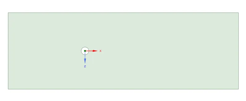
  • Of the cylinder which is a circle in our case is 2m
  • We will record the data for air incoming at different velocity from left to right we will change the velocity of air to record different Reynolds no. the viscosity and the density of the fluid will be constant
• Mesh –
  • In this case mesh needs to be very fine as we need to capture a detail simulation, so we are using a finer mesh of triangular type
• 
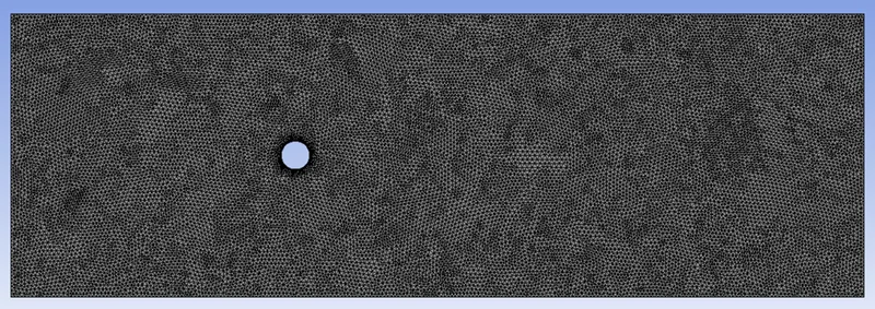
• As the mesh is really fine there are some more details added to get the simulation more accurate, like a body fitted mesh is created around the circle to achieve proper smooth cylinder from which air is flowing as shown in figure below

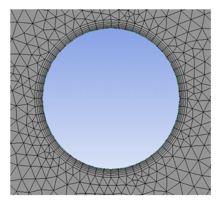
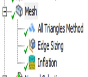
• Also, the inflation layers were added to the cylinder to capture the details at the point where actual physics was changing, even the mesh was made finer at the cylinder area

MATRIX POINT: -

• One mor detail which was added in simulation is a matrix point just after the cylinder, for around 10m from cylinder to the right, as shown in fig.

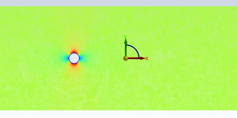
• All the velocity graph are of the velocity at this point as the actual changes are happening just behind the cylinder

CASE I: -

INPUT:

• Reynolds no. = 100
• Velocity = 2.5
• Type of solving = Steady State

OUTPUT: -

• As we are solving with steady state so there is no time component involved, so the oscillations in in lift coefficient cannot be calculated with particular time factor so the calculation and graphs are as follow

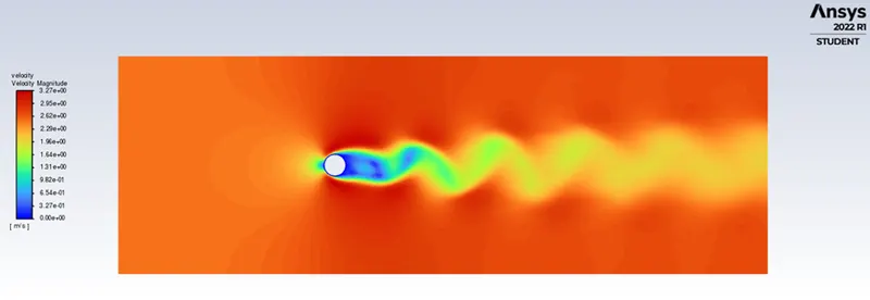
Vertex sheading velocity contours

• So, vertex sheading is clearly seen in this contour for Re = 100

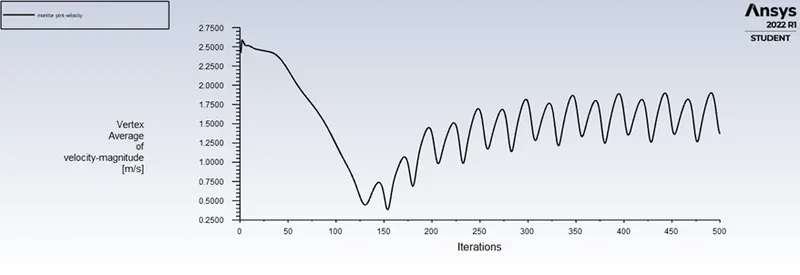
Velocity

• Oscillation of the velocity can be seen from which we can calculate the frequency to calculate Strouhal no.

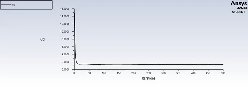
Drag coefficient

• For Reynolds no. 100 drag coefficient is constant and not oscillating

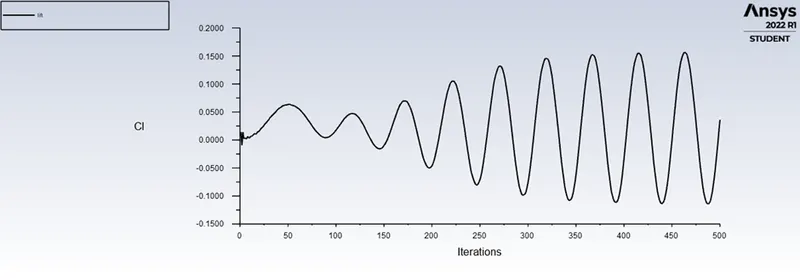
Lift coefficient

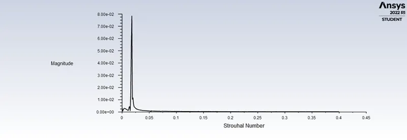
Strouhal’s no. graph

• Here, the Strouhal no. is at the maximum magnitude after writing it the Strouhal’s no. for this case is 0.79, Which is no correct according to the documented paper of ELSEVIR, the reason for that can be noted as there is no time involved in this simulation so the frequency cannot be calculated accurately

INPUT:

• Reynolds no. = 100
• Velocity = 2.5
• Type of solving = Iterative Method

OUTPUT:

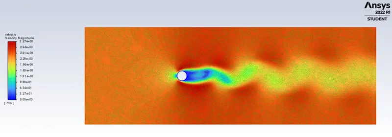
Vertex sheading

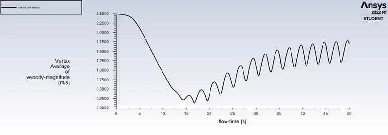
Velocity plot

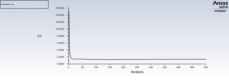
Drag coefficient

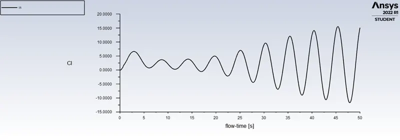
Lift coefficient

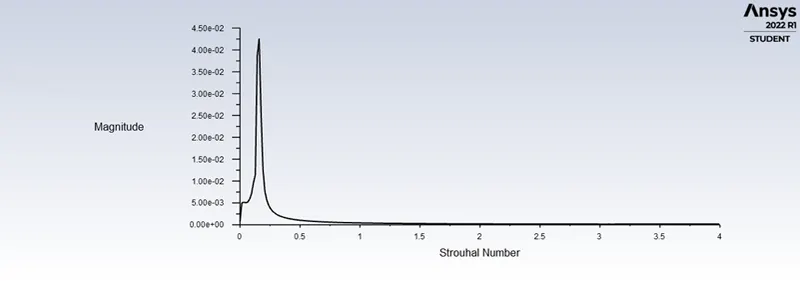
Strouhal number

• In this case the time is taken in consideration and so we can see good Oscillating movement in velocity and lift coefficient plot which can be calculated as, there is time factor involved
• Also, in this case the Strouhal’s no. can be calculated accurately so after writing the data from the above FFT plot we can see the following magnitudes

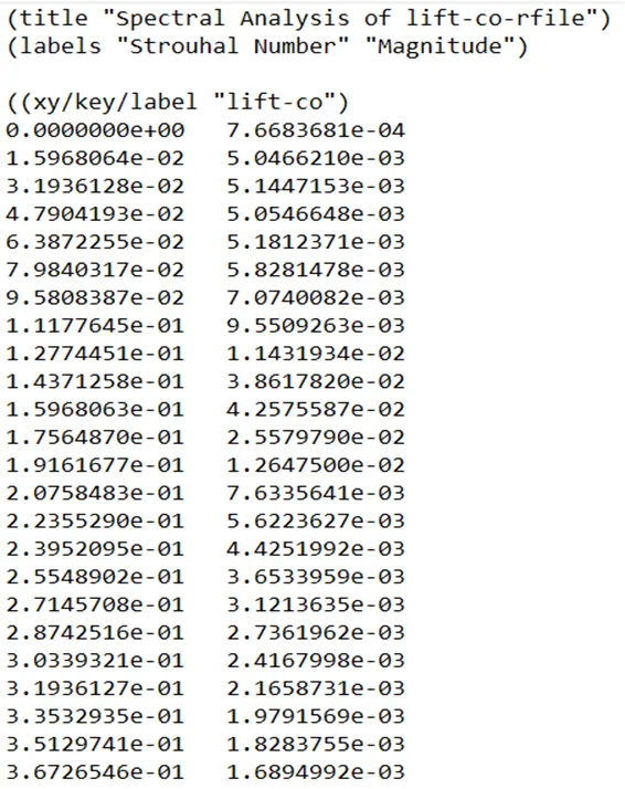
• The right column is magnitude and the highest magnitude is of 4.25*e^-2. The Strouhal’s no. value associated with it is 0.157. which can be validated from the documented paper

Result Table:

Re	Velocity	Method of Solving	cof. Of drag	Strouhal’s no	Published Value (Validation)
100	2.5	Steady	1.337	0.07	N/a
100	2.5	Iterative	1.328	0.153	0.156

Part II:

Now, for the calculations with diff. Re

• 1) Reynolds no. = 10

Here Vertex shedding was not present as the Reynolds no. is very low

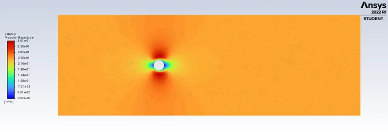
velocity contours

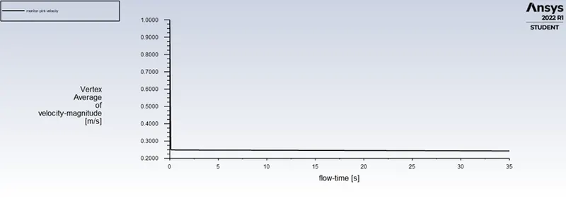
Velocity

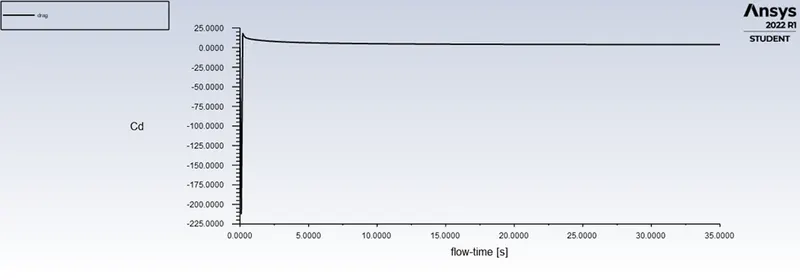
Drag coefficient

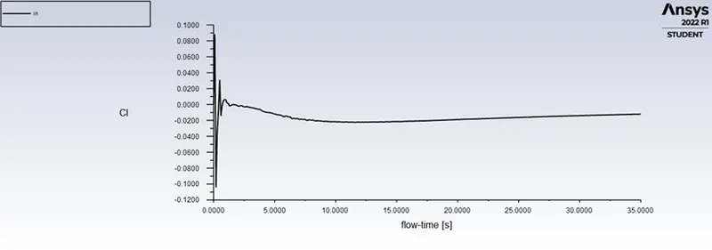
Lift coefficient

• As, all the values have rich at stable state we can say that the flow has converged
• 2) Reynolds no = 1000

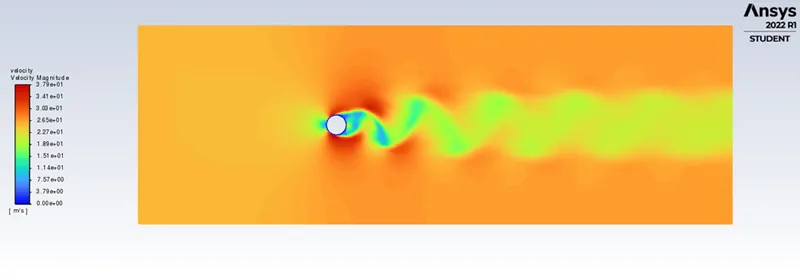
Vertex shedding

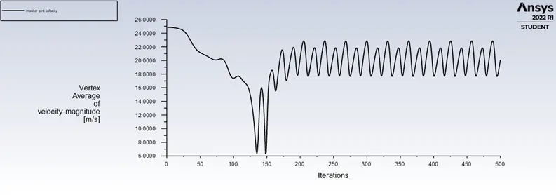
Velocity plot

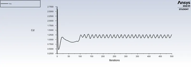
Drag coefficient

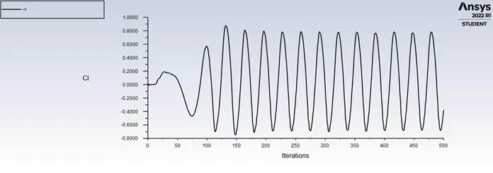
Lift coefficient

• In this process the major change we can spot is the coefficient of Drag is oscillating in a certain frequency which states that as the Reynolds no. increases the drag on the cylinder starts to increase and if not in its permittable values it can cause in failure
• Other thing also shows some massive changes as the lift coefficient is also very high
• As all the quantities are in recurring oscillations, we can say that the flow is converged

• 3) Reynolds no. = 10000

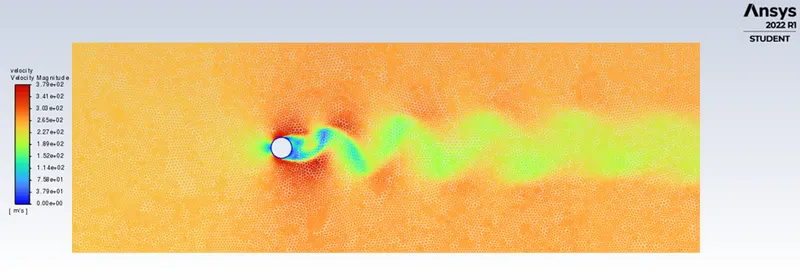
Vertex Shedding

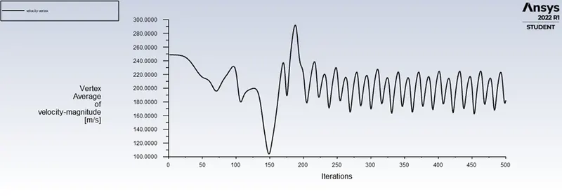
Velocity Plot

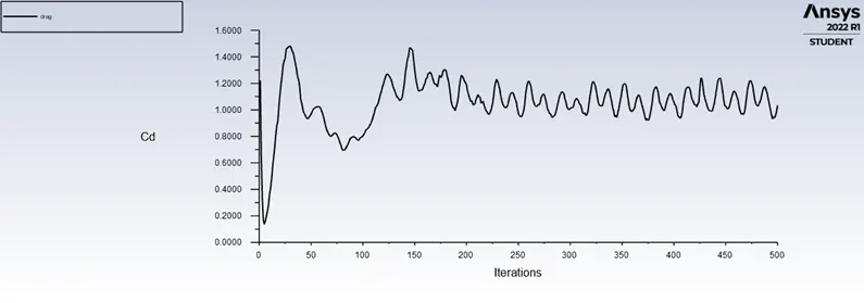
Drag coefficient

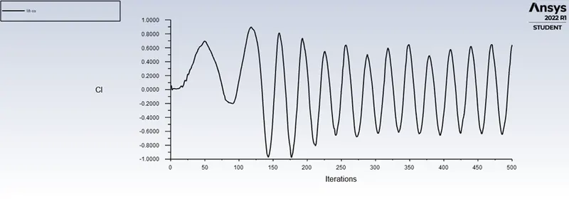
Lift coefficient

• The Coefficient of Drag is oscillating at a bigger frequency so we can state that with increase in Reynolds no. the coefficient of drag can increase its frequency of oscillating which if not measured properly can cause failure of the cylinder
• All the quantities are at converged as they are moving in a fixed patter ahead in iterations

• 4) Reynolds no = 100000

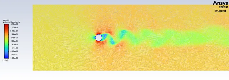
Velocity contours

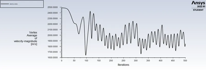
Velocity plot

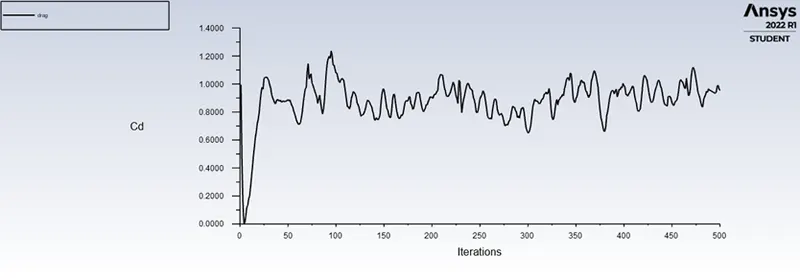
Drag coefficient

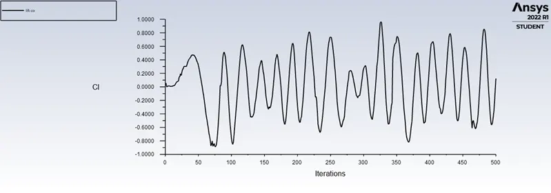
Lift coefficient

• The Magnitude of the drag and lift coefficient is increasing with increasing Reynolds no. Also, with so high Reynolds no. we can see the pattern of oscillation is not constant maybe, with more no. of iteration we can find the pattern in oscillations

Final Result Table:

Re no	Velocity	Coefficient of Drag (Mean)	Coefficient of Lift (Mean)
10	0.25	3.77	0.012
1000	25	1.22	0.015
10000	250	1.26	0.036
100000	2500	N/A	N/A

Conclusion:

• Vertex shedding happens when Reynolds no exceeds 100, When Re increases the Coefficient of Drag also starts to oscillate in certain magnitude, The magnitude is directly proportional to Reynolds no.
• The Strouhal no. can be validated in iterative method, the Literature I used for validation is ELSIVIERhttps://www.sciencedirect.com/science/article/pii/S0307904X08000243