Week 11 - Simulation of Flow through a pipe in OpenFoam

Hagen- Poiseuille's equation is very important equation with many applications, it basically suggests how the flow can be affected by various factors.

By experiments it the equation was derived which eventually stated that, flow(Q) is directly proportional to change in pressure

and inversely proportional to length of pipe and viscosity of fluid

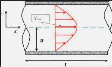
As shown in fig. the Velocity is max in middle of the pipe and lowest at the walls as the shear stress is maximum at the end of pipe and lowest at the middle

In my Simulation, the input is as follow

Length = 1.5

Dia. of pipe = 0.01 m

Reynolds no. = 2100

Inlet Velocity = 0.2m/s

Density = 997 kg/m^3

So by, Hydro-dynamic length = 0.06*D*Re = 1.2m

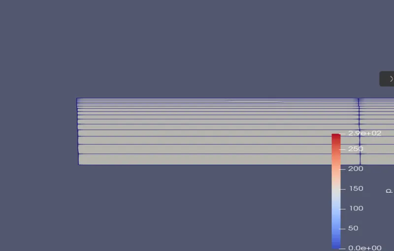
This is how my mesh looks like it is finer where boundary layer is form in pipe

So, the following Graph shows how the graph for velocity changes with length, and turns into our actual analytical parabolic shape,

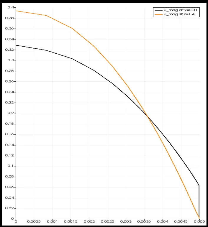
The black line shows how the graph looks before Hydro-dynamic lenghth and the yellow graph shows how the velocity will look after the hydro-dynamic length is covered

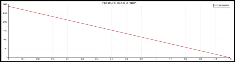
Similarly the pressure drops through the pipe as we have assumed that at the outlet the pressure is atmospheric pressure and at the inlet it needs to be slightly higher as the fluid to flow

The following graph shows how the pressure drops through the length of pipe

now,

For validating our derived ans, Vmax = 2 . Vavg

Our Vavg = 0.2 Therefore, Vmax = 0.4 m/s, and the ans can be seen in our graph as the complete parabolic shape is achived the Vmax = 0.4

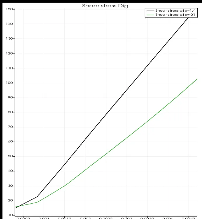
The Following graph shows the shear stress dig. as it is maximum at the wall of pipe and minimum at the centre of the pipe

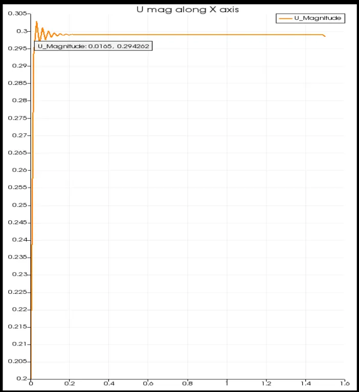
HP equation shows how the flow can be calculated i.e. in l/s how much fluid can be flowed through the pipe, the following chart shows the velocity flow through the length of pipe how the discontinuities in the start are then normalised with change in pressure