Curve fitting using Python
Aim: To perform curve fitting using Python.
Objective:
- Write codes to fit the linear and cubic polynomial for Cp data.
- To plot the linear and cubic fit curves along with the original data points.
- To find the best fit and measure the errors in the curves.
Curve fitting:
Curve fitting is the process of constructing a curve or mathematical function, that has the best fit to a series of data points, possibly subject to constraints. Curve fitting can involve either interpolation, where an exact fit to the data is required, or smoothing, in which a "smooth" function is constructed that approximately fits the data. A related topic is regression analysis, which focuses more on questions of statistical inference such as how much uncertainty is present in a curve that is fit to data observed with random errors. Fitted curves can be used as an aid for data visualization, to infer values of a function where no data are available, and to summarize the relationships among two or more variables. Extrapolation refers to the use of a fitted curve beyond the range of the observed data and is subject to a degree of uncertainty since it may reflect the method used to construct the curve as much as it reflects the observed data.
Linear curve fitting, or linear regression, is when the data is fit to a straight line. Although there might be some curve to your data, a straight line provides a reasonable enough fit to make predictions. Since the equation of a generic straight line is always given by f(x)= a x + b, the question becomes: what a and b will give us the best fit line for our data?
Considering the vertical distance from each point to a prospective line as an error, and summing them up over our range, gives us a concrete number that expresses how far from ‘best’ the prospective line is.
A line that provides a minimum error can be considered the best straight line.
Since it’s the distance from our points to the line we’re interested in—whether it is positive or negative distance is not relevant—we square the distance in our error calculations. This also allows us to weigh greater errors more heavily. So this method is called the least-squares approach.
Polynomial curve fitting is when we fit our data to the graph of a polynomial function. The same least-squares method can be used to find the polynomial, of a given degree, that has a minimum total error.
Upon finding a curve that satisfies the data points there are 4 quantities that help us measure the goodness of fit criteria or how well the equation is representing the data points. There are,
The sum of squares due to error (SSE)
R-square
Adjusted R-square
Root mean squared error (RMSE).
Equations to be used:
Error = `|y(i) - f(x(i))|`
`SSE`(Sum of Squared Errors) = `sum_(i=1)^n`Error`(i)^2`
`SSR`(Sum of Squared Regression) = `sum_(i=1)^n (f(x(i)) - mean)^2`
`SST = SSE+SSR`
`R^2 = (SSR)/(SST`
`RMSE = sqrt((SSE)/n)`
Python Code:
import math
import matplotlib.pyplot as plt
from scipy.optimize import curve_fit
import numpy as np

# Curve fitting with linear equation

def func_0(t,a,b):
	return a*t + b

# Curve fitting with quadratic equation
def func_1(t,a,b,c):
	return a*pow(t,2) + b*t + c

# Curve fitting with cubic equation
def func_2(t,a,b,c,d):
	return a*pow(t,3) + b*pow(t,2) + c*t + d

# Curve fitting with quartic equation
def func_3(t,a,b,c,d,e):
	return a*pow(t,4) + b*pow(t,3) + c*pow(t,2) + d*t + e


def read_file():
	temperature = []
	cp = []
	for line in open('data','r'):
		values = line.split(',')
		temperature.append(float(values[0]))
		cp.append(float(values[1]))
	return [temperature,cp]

temperature,cp = read_file()
popt , pcov = curve_fit(func_0,temperature,cp)
fit_cp = func_0(np.array(temperature), *popt)

# plotting the results for linear equation
plt.figure(1)
plt.plot(temperature,cp,color ='green',linewidth = 3)
plt.plot(temperature,fit_cp,color = 'red',linewidth = 3)
plt.legend(['Actual data','Curve fit'])
plt.xlabel('Temperature')
plt.ylabel('Cp')
plt.title('Curve fitting using Linear polynomial')
plt.show()

popt_1 , pcov_1 = curve_fit(func_1,temperature,cp)
fit_cp_1 = func_1(np.array(temperature), *popt_1)

# plotting the results for quadratic equation
plt.figure(2)
plt.plot(temperature,cp,color ='green',linewidth = 3)
plt.plot(temperature,fit_cp_1,color = 'red',linewidth = 3)
plt.legend(['Actual data','Curve fit'])
plt.xlabel('Temperature')
plt.ylabel('Cp')
plt.title('Curve fitting using Quadratic polynomial')
plt.show()


popt_2 , pcov_2 = curve_fit(func_2,temperature,cp)
fit_cp_2 = func_2(np.array(temperature), *popt_2)

# plotting the results for cubic equation
plt.figure(3)
plt.plot(temperature,cp,color ='green',linewidth = 3)
plt.plot(temperature,fit_cp_2,color = 'red',linewidth = 3)
plt.legend(['Actual data','Curve fit'])
plt.xlabel('Temperature')
plt.ylabel('Cp')
plt.title('Curve fitting using Cubic polynomial')
plt.show()

popt_3 , pcov_3 = curve_fit(func_3,temperature,cp)
fit_cp_3 = func_3(np.array(temperature), *popt_3)

# plotting the results for quartic equation
plt.figure(4)
plt.plot(temperature,cp,color ='green',linewidth = 3)
plt.plot(temperature,fit_cp_3,color = 'red',linewidth = 3)
plt.legend(['Actual data','Curve fit'])
plt.xlabel('Temperature')
plt.ylabel('Cp')
plt.title('Curve fitting using Quartic polynomial')
plt.show()


# Now we need to find out the characterstics of the curve.
# In other words we need to find out which curve has the best fit mathematically.
"""
ssr = sum pf squares regression
sse = sum of squared errors
sst = ssr + sse
R_square = ssr/sst
RMSE = (sse/n)*0.5
"""

s = np.sum(cp) # Sum of all the values of cp
n = len(cp) # Number of cp values

mean = s/n # Mean of cp

# For Linear curve fit

linear_ssr = 0
linear_sse = 0

for i in range(n):
	linear_error = abs(np.sum(cp[i] - fit_cp[i]))
	linear_sse = linear_sse + pow(linear_error,2)
	linear_ssr = linear_ssr + np.sum(pow((fit_cp[i] - mean),2))

SSR_1 = linear_ssr
SSE_1 = linear_sse

SST_1 = SSR_1 + SSE_1

R_square_1 = SSR_1/SST_1

RMSE_1 = pow((SSE_1/n),0.5)

print('The value of R_square for the Linear polynomial is:',R_square_1)
print('nThe value of Root Mean Square Error(RMSE) for Linear polynomial :',RMSE_1)

# For Quadratic curve fit

quadratic_ssr = 0
quadratic_sse = 0

for j in range(n):
	quadratic_error = abs(np.sum(cp[j] - fit_cp_1[j]))
	quadratic_sse = quadratic_sse + pow(quadratic_error,2)
	quadratic_ssr = quadratic_ssr + np.sum(pow((fit_cp_1[j] - mean),2))

SSR_2 = quadratic_ssr
SSE_2 = quadratic_sse

SST_2 = SSR_2 + SSE_2

R_square_2 = SSR_2/SST_2

RMSE_2 = pow((SSE_2/n),0.5)

print('nThe value of R_square for the Quadratic polynomial is:',R_square_2)
print('nThe value of Root Mean Square Error(RMSE) for Quadratic polynomial :',RMSE_2)

# For Cubic curve fit

cubic_ssr = 0
cubic_sse = 0

for k in range(n):
	cubic_error = abs(np.sum(cp[k] - fit_cp_2[k]))
	cubic_sse = cubic_sse + pow(cubic_error,2)
	cubic_ssr = cubic_ssr + np.sum(pow((fit_cp_2[k] - mean),2))

SSR_3 = cubic_ssr
SSE_3 = cubic_sse

SST_3 = SSR_3 + SSE_3

R_square_3 = SSR_3/SST_3

RMSE_3 = pow((SSE_3/n),0.5)

print('nThe value of R_square for the Cubic polynomial is:',R_square_3)
print('nThe value of Root Mean Square Error(RMSE) for Cubic polynomial :',RMSE_3)

# For Quartic curve fit

quartic_ssr = 0
quartic_sse = 0

for l in range(n):
	quartic_error = abs(np.sum(cp[l] - fit_cp_3[l]))
	quartic_sse = quartic_sse + pow(quartic_error,2)
	quartic_ssr = quartic_ssr + np.sum(pow((fit_cp_3[l] - mean),2))

SSR_4 = quartic_ssr
SSE_4 = quartic_sse

SST_4 = SSR_4 + SSE_4

R_square_4 = SSR_4/SST_4

RMSE_4 = pow((SSE_4/n),0.5)

print('nThe value of R_square for the Quartic polynomial is:',R_square_4)
print('nThe value of Root Mean Square Error(RMSE) for Quartic polynomial :',RMSE_4)
Results:
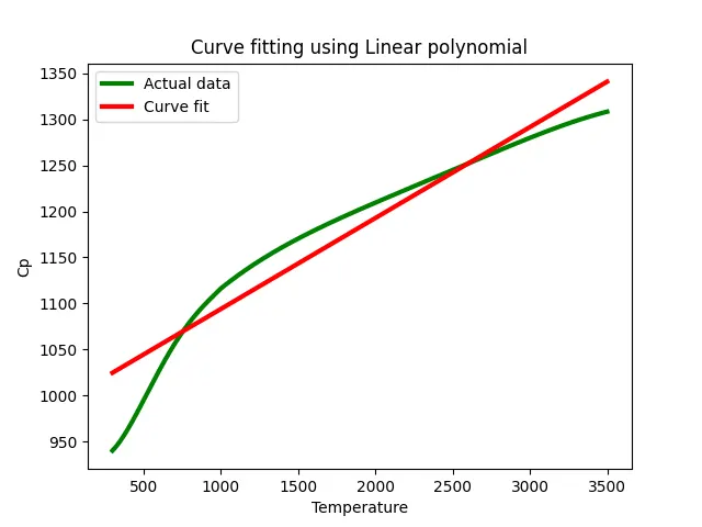
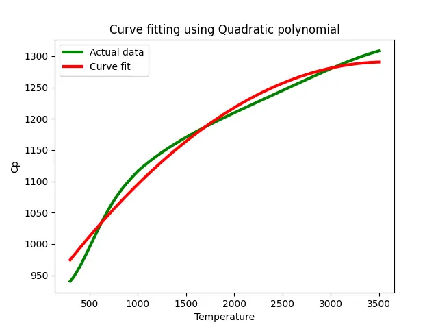
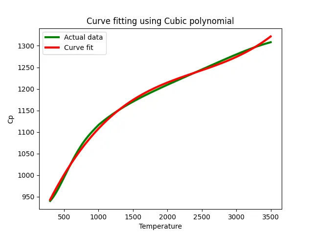
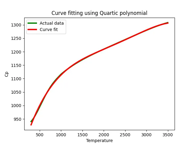
The value of R_square for the Linear polynomial is: 0.9248776260524184

The value of Root Mean Square Error(RMSE) for Linear polynomial : 25.999093068195325

The value of R_square for the Quadratic polynomial is: 0.9812421444745516

The value of Root Mean Square Error(RMSE) for Quadratic polynomial : 12.991674772728752

The value of R_square for the Cubic polynomial is: 0.996725946714689

The value of Root Mean Square Error(RMSE) for Cubic polynomial : 5.42770728878495

The value of R_square for the Quartic polynomial is: 0.9996155309982948

The value of Root Mean Square Error(RMSE) for Quartic polynomial : 1.8599626013389154
[Finished in 51.5s]
Conclusion:
The Value of R_square is greatest in quartic equation and the value of RMSE is lowest in quartic equation so in this way visually and mathematically Quartic equation corresponds to the best fit.
Now based on this excercise we need to answer some of the questions asked in the challenge:
1. What does popt and pcov mean? (Watch the video to get some context)
Ans: 'popt' represents the matrix which stores and extracts the coecients for the tting functions according to the general equations dened.
popt : array, Optimal values for the parameters so that the sum of the squared residuals of f(xdata, *popt) - ydata is minimized.
'pcov' represents the square matrix which stores the estimated values of covariance of the coecients of the above. The diagonal element of this square matrix also represents variance of that coefficients.
pcov : 2d array.
2. What does np.array(temperature) do?
Ans: This command converts each value of temperature in the data file into an array using numpy module.
3. What does the * in *popt mean?
Ans: '*' , '*popt' indicates and returns each coefficients stored in popt array.
4. What needs to be done in order to make the curve fit perfect?
Ans: If we increase the order of the polynomial, the error produced will be less and curve fit perfectly. On increasing the order of the polynomial the value of will be close to 1 and is assumed to perfect fit.