Simulation of Flow through a pipe in OpenFoam
Objective:
- Simulating flow in a circular pipe in OpenFoam.
- Writing a MATLAB program to automate the generation of the blockMeshDict file for the circular pipe.
- Validating the simulation results using Hagen- Poiseuille's equation for the fully developed flow.
Problem Statement:
The flow is laminar and flows through a constant cross-section pipe at an inlet Reynold's number of 2100. We can do a transient or steady state simulation and you will validate your results with the Hagen- Poiseuille's equations for the fully developed flow.
We will also write code in Matlab to automate the generation of blockMeshDict file. The code should take inputs like pipe length, diameter, wedge angle, etc and output a fully functional blockMeshDict file.
Expected Results
- Validate Hydro-dynamic length with the numerical result
- Validate the fully developed flow velocity profile with its analytical profile
- Validate maximum velocity and pressured drop for fully developed flow
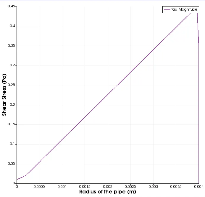
- Post-process Shear stress and validate wall shear stress for fully developed flow.
Hagen-Poiseuille's equation:
In nonideal fluid dynamics, the Hagen–Poiseuille equation, also known as the Hagen–Poiseuille law, Poiseuille law or Poiseuille equation, is a physical law that gives the pressure drop in an incompressible and Newtonian fluid in laminar flow flowing through a long cylindrical pipe of constant cross section. It can be successfully applied to air flow in lung alveoli, or the flow through a drinking straw or through a hypodermic needle. It was experimentally derived independently by Jean Léonard Marie Poiseuille in 1838 and Gotthilf Heinrich Ludwig Hagen, and published by Poiseuille in 1840–41 and 1846. The theoretical justification of the Poiseuille law was given by George Stokes in 1845.
The assumptions of the equation are that the fluid is incompressible and Newtonian; the flow is laminar through a pipe of constant circular cross-section that is substantially longer than its diameter; and there is no acceleration of fluid in the pipe. For velocities and pipe diameters above a threshold, actual fluid flow is not laminar but turbulent, leading to larger pressure drops than calculated by the Hagen–Poiseuille equation.
Poiseuille's Equation describes the pressure drop due to the viscosity of the fluid; Other types of pressure drops may still occur in a fluid (see a demonstration here). For example, the pressure needed to drive a viscous fluid up against gravity would contain both that as needed in Poiseuille's Law plus that as needed in Bernoulli's equation, such that any point in the flow would have a pressure greater than zero (otherwise no flow would happen).
Another example is when blood flows into a narrower constriction, its speed will be greater than in a larger diameter (due to continuity of volumetric flow rate), and its pressure will be lower than in a larger diameter (due to Bernoulli's equation). However, the viscosity of blood will cause additional pressure drop along the direction of flow, which is proportional to length traveled (as per Poiseuille's Law). Both effects contribute to the actual pressure drop.
In standard fluid-kinetics notation:
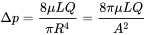
- Δ p = 8 μ L Q π R 4 = 8 π μ L Q A 2 {displaystyle Delta p={frac {8mu LQ}{pi R^{4}}}={frac {8pi mu LQ}{A^{2}}}}
where:
- Δp is the pressure difference between the two ends,
- L is the length of pipe,
- μ is the dynamic viscosity,
- Q is the volumetric flow rate,
- R is the pipe radius,
- A is the cross section of pipe.
1. Pre-Processing:
In this step we will be creating an OpenFoam file and then built the geometry of a wedge of the circular pipe.
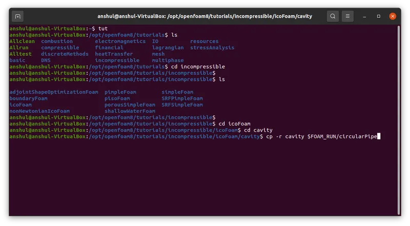
To do that we will first copy the required file from the tutorials of the OpenFoam and create a different file in different folder.
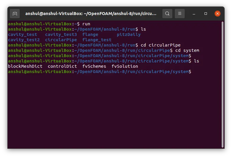
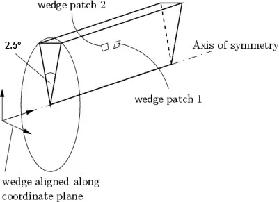
Now we need to generate a blockMeshDict file using MATLAB to create the geometry of a wedge of the circular pipe. But we need make some assumptions for the input values.
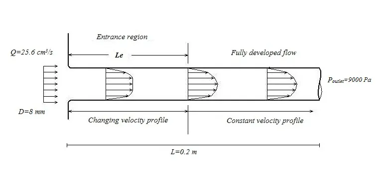
The wedge of the circular pipe should be represented as shown in fig below:
Assumptions:
- Incompressible flow.
- Laminar flow.
- Newtonian flow.
- Cylindrical symmetry.
- Negligible gravity effects.
- Steady flow.
- Very large pipe so that when flow becomes fully developed, `v_z ne 0` but `v_theta =0` and `v_r =0`.
- Smooth pipe so that roughness does not influence.
File Writing in MATLAB;
We will create a function named as blockMesh so that we can use it in the main program where all the inputs will be mentioned.
function [f1] = blockMesh(R,theta,L,nx,ny,nz)
% Writing  blockMeshDict file for OpenFoam
f1 = fopen('blockMeshDict','w');
% Intro of the file
fprintf(f1,"/*--------------------------------*- C++ -*----------------------------------*n");
fprintf(f1,'  =========                 | n');
fprintf(f1,'  \      /  F ield         | OpenFOAM: The Open Source CFD Toolbox n');
fprintf(f1,'   \    /   O peration     | Website:  https://openfoam.org n');
fprintf(f1,'    \  /    A nd           | Version:  8 n');
fprintf(f1,'     \/     M anipulation  | n');
fprintf(f1,'*---------------------------------------------------------------------------*/ n');
fprintf(f1,'FoamFile n');
fprintf(f1,'{ n');
fprintf(f1,'    version     2.0; n');
fprintf(f1,'   format      ascii; n');
fprintf(f1,'    class       dictionary; n');
fprintf(f1,'    object      blockMeshDict; n');
fprintf(f1,'} n');
fprintf(f1,'// * * * * * * * * * * * * * * * * * * * * * * * * * * * * * * * * * * * * * // n');
fprintf(f1,'n');
fprintf(f1,'convertToMeters 0.001; n');
fprintf(f1,'n');
fprintf(f1,'verticesn');
% Verteces of the wedge geometry
fprintf(f1,'( n');
fprintf(f1,'    (0 0 0) // Vertex 0 n');
fprintf(f1,'    (0 %f %f) // Vertex 1 n',R*cosd(theta/2),-R*sind(theta/2));
fprintf(f1,'    (0 %f %f) // Vertex 2 n',R*cosd(theta/2),R*sind(theta/2));
fprintf(f1,'    (%d 0 0) // Vertex 3 n',L);
fprintf(f1,'    (%d %f %f) // Vertex 4 n',L,R*cosd(theta/2),-R*sind(theta/2));
fprintf(f1,'    (%d %f %f) // Vertex 5 n',L,R*cosd(theta/2),R*sind(theta/2));
fprintf(f1,'); n');

% Blocks
fprintf(f1,'blocks n');
fprintf(f1,'( n');
fprintf(f1,'    hex (0 1 2 0 3 4 5 3) (%d %d %d) simpleGrading (0.1 1 10) n',nx,ny,nz);
fprintf(f1,'); n');

% Edges
fprintf(f1,'n');
fprintf(f1,'edges n');
fprintf(f1,'( n');
fprintf(f1,'   arc 1 2 (0 %d 0) n',R);
fprintf(f1,'   arc 4 5 (%d %d 0) n',L,R);
fprintf(f1,'); n');

%Boundary
fprintf(f1,'n');
fprintf(f1,'boundary n');
fprintf(f1,'( n');
%Axis
fprintf(f1,'   axis n');
fprintf(f1,'   {n');
fprintf(f1,'     type empty; n');
fprintf(f1,'     facesn');
fprintf(f1,'     (n');
fprintf(f1,'            (0 3 3 0) n');
fprintf(f1,'     );n');
fprintf(f1,'   }n');
fprintf(f1,'n');
%Inlet
fprintf(f1,'   inletn');
fprintf(f1,'   {n');
fprintf(f1,'     type patch; n');
fprintf(f1,'     facesn');
fprintf(f1,'     (n');
fprintf(f1,'            (0 0 2 1) n');
fprintf(f1,'     );n');
fprintf(f1,'   }n');
fprintf(f1,'n');
% Wall
fprintf(f1,'   walln');
fprintf(f1,'   {n');
fprintf(f1,'     type wall; n');
fprintf(f1,'     facesn');
fprintf(f1,'     (n');
fprintf(f1,'            (2 5 4 1) n');
fprintf(f1,'     );n');
fprintf(f1,'   }n');
fprintf(f1,'n');
%Outlet
fprintf(f1,'   outletn');
fprintf(f1,'   {n');
fprintf(f1,'     type patch; n');
fprintf(f1,'     facesn');
fprintf(f1,'     (n');
fprintf(f1,'            (3 4 5 3) n');
fprintf(f1,'     );n');
fprintf(f1,'   }n');
fprintf(f1,'n');
% Front
fprintf(f1,'   frontn');
fprintf(f1,'   {n');
fprintf(f1,'     type wedge; n');
fprintf(f1,'     facesn');
fprintf(f1,'     (n');
fprintf(f1,'            (0 3 5 2) n');
fprintf(f1,'     );n');
fprintf(f1,'   }n');
fprintf(f1,'n');
% Back
fprintf(f1,'   backn');
fprintf(f1,'   {n');
fprintf(f1,'     type wedge; n');
fprintf(f1,'     facesn');
fprintf(f1,'     (n');
fprintf(f1,'            (0 1 4 3) n');
fprintf(f1,'     );n');
fprintf(f1,'   }n');
fprintf(f1,'n');
fprintf(f1,'); n');
% Ending the file
fprintf(f1,'n');
fprintf(f1,'mergePatchPairs n');
fprintf(f1,'(n');
fprintf(f1,');n');
fprintf(f1,'n');
fprintf(f1,'// ************************************************************************* //');
end
Main Program:
clear all
close all
clc

% Inputs
L = 200; % Length of the pipe in mm
Re = 2100; % Reynolds Number
D = 8; % Diameter of the pipe in mm
theta = 2.5; %angle of the wedge in degrees.
rho = 997; % density in kg/m3.
R = D/2; %Radius of the pipe
mu = 8.97e-4; %Dynamic Viscosity Pa.s

nx = 50;
ny = 1;
nz = 500;

file = blockMesh(R,theta,L,nx,ny,nz);
Output:
/*--------------------------------*- C++ -*----------------------------------*
  =========                 |
        /  F ield         | OpenFOAM: The Open Source CFD Toolbox
       /   O peration     | Website:  https://openfoam.org
      /    A nd           | Version:  8
     /     M anipulation  |
*---------------------------------------------------------------------------*/
FoamFile
{
    version     2.0;
   format      ascii;
    class       dictionary;
    object      blockMeshDict;
}
// * * * * * * * * * * * * * * * * * * * * * * * * * * * * * * * * * * * * * //

convertToMeters 0.001;

vertices
(
    (0 0 0) // Vertex 0
    (0 3.999048 -0.087260) // Vertex 1
    (0 3.999048 0.087260) // Vertex 2
    (200 0 0) // Vertex 3
    (200 3.999048 -0.087260) // Vertex 4
    (200 3.999048 0.087260) // Vertex 5
);
blocks
(
    hex (0 1 2 0 3 4 5 3) (50 1 500) simpleGrading (0.1 1 10)
);

edges
(
   arc 1 2 (0 4 0)
   arc 4 5 (200 4 0)
);

boundary
(
   axis
   {
     type empty;
     faces
     (
            (0 3 3 0)
     );
   }

   inlet
   {
     type patch;
     faces
     (
            (0 0 2 1)
     );
   }

   wall
   {
     type wall;
     faces
     (
            (2 5 4 1)
     );
   }

   outlet
   {
     type patch;
     faces
     (
            (3 4 5 3)
     );
   }

   front
   {
     type wedge;
     faces
     (
            (0 3 5 2)
     );
   }

   back
   {
     type wedge;
     faces
     (
            (0 1 4 3)
     );
   }

);

mergePatchPairs
(
);

// ************************************************************************* //
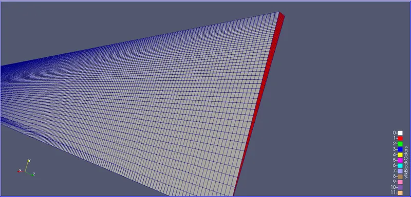
Now copy and paste this blockMeshDict file inside the circularPipe folder in OpenFoam.
When running blockMeshDict file ,the mesh generated is shown below.
Boundary and Initial Conditions:
When solving circulating internal flow, the most common boundary conditions are to fix an inlet velocity and an outlet pressure or vice-versa.
/*--------------------------------*- C++ -*----------------------------------*
  =========                 |
  \      /  F ield         | OpenFOAM: The Open Source CFD Toolbox
   \    /   O peration     | Website:  https://openfoam.org
    \  /    A nd           | Version:  8
     \/     M anipulation  |
*---------------------------------------------------------------------------*/
FoamFile
{
    version     2.0;
    format      ascii;
    class       volScalarField;
    object      p;
}
// * * * * * * * * * * * * * * * * * * * * * * * * * * * * * * * * * * * * * //

dimensions      [0 2 -2 0 0 0 0];

internalField   uniform 0;

boundaryField
{
    axis
    {
        type            empty;
    }

    inlet
    {
        type            zeroGradient;
    }

    wall
    {
        type            zeroGradient;
    }
    outlet
    {
        type            fixedValue;
        value		 uniform 10;
    }
    front
    {
        type            wedge;
    }
    back
    {
        type            wedge;
    }
}

// ************************************************************************* //
/*--------------------------------*- C++ -*----------------------------------*
========= |
\ / F ield | OpenFOAM: The Open Source CFD Toolbox
\ / O peration | Website: https://openfoam.org
\ / A nd | Version: 8
\/ M anipulation |
*---------------------------------------------------------------------------*/
FoamFile
{
version 2.0;
format ascii;
class volVectorField;
object U;
}
// * * * * * * * * * * * * * * * * * * * * * * * * * * * * * * * * * * * * * //
dimensions [0 1 -1 0 0 0 0];
internalField uniform (0.50929 0 0);
boundaryField
{
axis
{
type empty;
}
inlet
{
type fixedValue;
value uniform (0.50929 0 0);
}
wall
{
type fixedValue;
value uniform (0 0 0);
}
outlet
{
type inletOutlet;
inletValue uniform (0.50929 0 0);
value uniform (0.50929 0 0);
}
front
{
type wedge;
}
back
{
type wedge;
}
}
// ************************************************************************* //The inlet velocity has been computed as:
`V = (Q)/(pi*(D/2)^2)` = `(25.6xx10^-6)/(pi*(4xx10^-3)^2)`
In the U dictionary one finds new type of boundary conditions called inletOutet . It switches p and U between fixedValue and zeroGradient: the first when the flow is ingoing and the second when the flow is outgoing.
Physical Properties:
/*--------------------------------*- C++ -*----------------------------------*
  =========                 |
  \      /  F ield         | OpenFOAM: The Open Source CFD Toolbox
   \    /   O peration     | Website:  https://openfoam.org
    \  /    A nd           | Version:  8
     \/     M anipulation  |
*---------------------------------------------------------------------------*/
FoamFile
{
    version     2.0;
    format      ascii;
    class       dictionary;
    location    "constant";
    object      transportProperties;
}
// * * * * * * * * * * * * * * * * * * * * * * * * * * * * * * * * * * * * * //

transportModel	 Newtonian;
nu              [0 2 -1 0 0 0 0] 0.000032;


// ************************************************************************* //
Control Dictionary:
/*--------------------------------*- C++ -*----------------------------------*
  =========                 |
  \      /  F ield         | OpenFOAM: The Open Source CFD Toolbox
   \    /   O peration     | Website:  https://openfoam.org
    \  /    A nd           | Version:  8
     \/     M anipulation  |
*---------------------------------------------------------------------------*/
FoamFile
{
    version     2.0;
    format      ascii;
    class       dictionary;
    location    "system";
    object      controlDict;
}
// * * * * * * * * * * * * * * * * * * * * * * * * * * * * * * * * * * * * * //

application     icoFoam;

startFrom       startTime;

startTime       0;

stopAt          endTime;

endTime         0.2;

deltaT          0.00005;

writeControl    timeStep;

writeInterval   20;

purgeWrite      0;

writeFormat     ascii;

writePrecision  6;

writeCompression off;

timeFormat      general;

timePrecision   6;

runTimeModifiable true;


// ************************************************************************* //
2. Post-Processing:
Results of the Simulation:
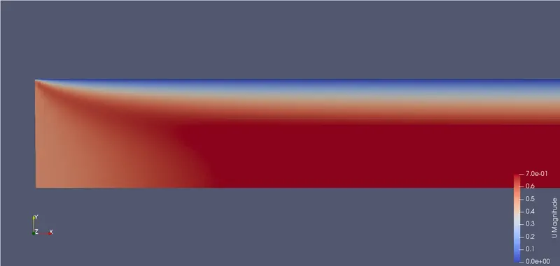
The velocity field at the inlet of the pipe (non-developed flow);
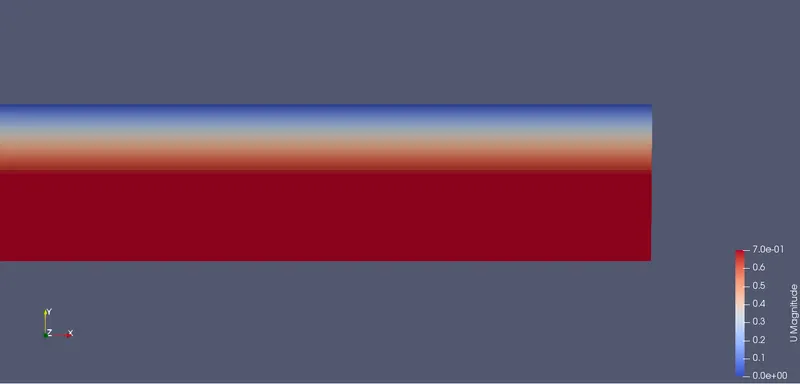
The velocity field at the outlet of the pipe (developed flow):
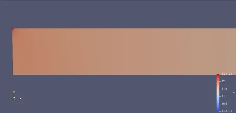
The pressure field along the pipe at inlet:
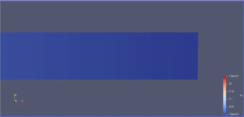
The pressure field along the pipe at outlet:
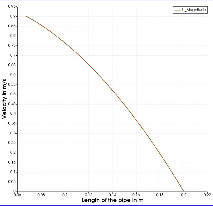
Variation of velocity of the flow along the length of the pipe:
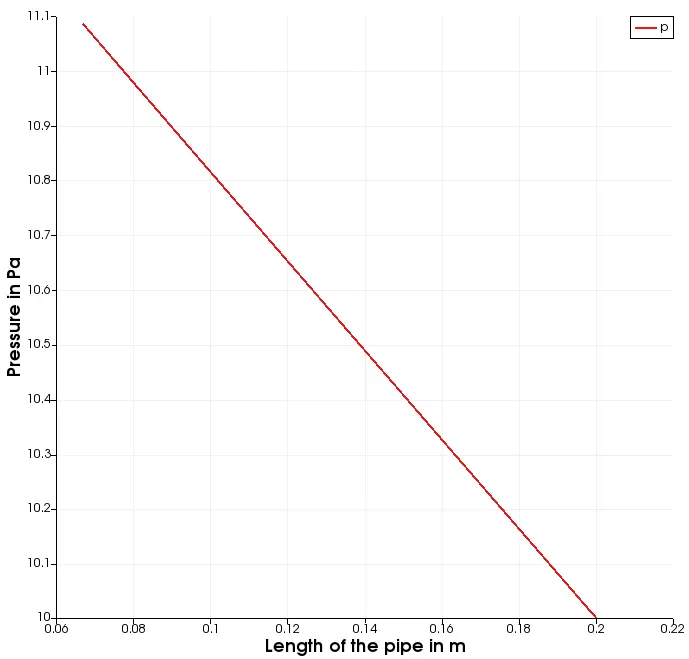
Variation of pressure of the flow along the length of the pipe:
Shear stress variation along the radius of the pipe:
3. Validating the results:
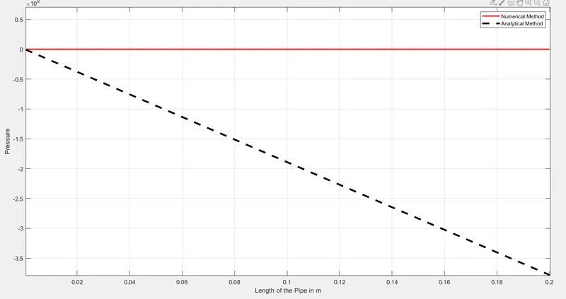
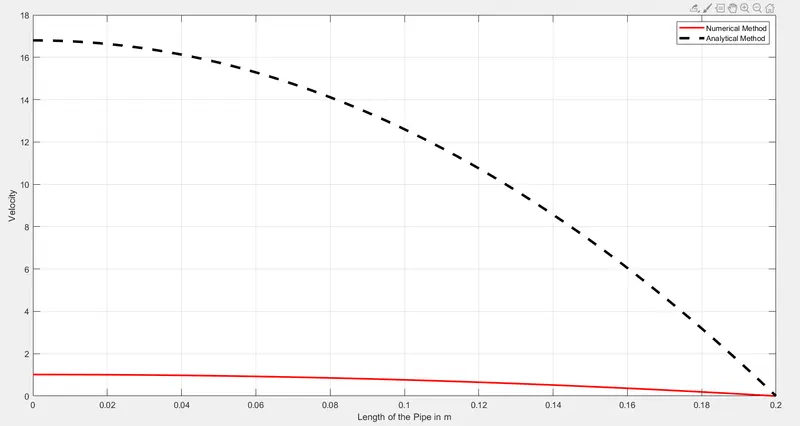
After the post processing of the model we need to validate the results obtained from the numerical analysis using Hagen-Poiseulle's equation in MATLAB.
But to do that we first need to collect the data from the openFoam in a spreadsheet then read it in MATLAB.
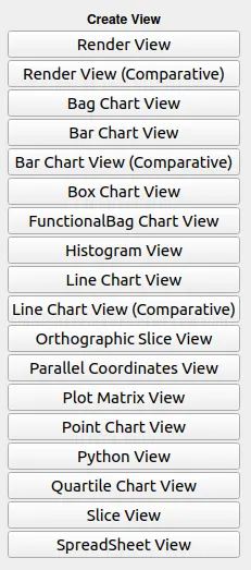
Choosing the Spreadsheet view option from the above, we get:
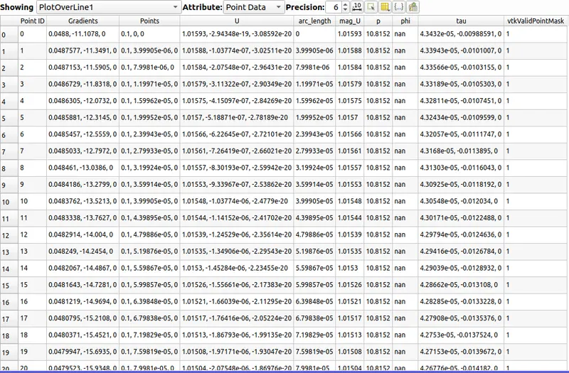
Now exporting this spreadsheet to the system and getting the file ready to read it in MATLAB.
File reading in MATLAB:
Now we are going to import the csv file using import data button in the MATLAB and import it as column vectors:
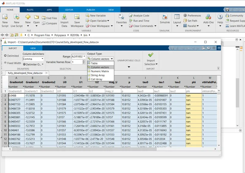
After importing thhe data we will calculate the analytical velocity and pressure compare the results with the numerical results.
% Inputs
Q = 25.6e-6;% Flow rate at inlet
L = 200; % Length of the pipe in mm
Re = 2100; % Reynolds Number
D = 8; % Diameter of the pipe in mm
theta = 2.5; %angle of the wedge in degrees.
rho = 900; % density in kg/m3.
R = D/2; %Radius of the pipe
mu = 0.0288; %Dynamic Viscosity Pa.s

nx = 50;
ny = 1;
nz = 500;

file = blockMesh(R,theta,L,nx,ny,nz);

% Calculation for Analytical Methods
Ln = linspace(0,0.2,1001);
r = linspace(0,0.004,1001);
Vn = mag_U;
Pn = p;

%Analytical Method for Velocity
V_avg = (Re*mu)/(rho*(D/1000));
V_r = 2*V_avg*(1-(r.^2/0.004^2));

% Analytical Method for Pressure drop
P = -(32*mu*Ln.*V_avg)/(0.008^4);

% Plotting for Validation between Numerical and Analytical method.
% Plot for Velocity
figure(1)
plot(Ln,Vn,'r','linewidth',2)
hold on
plot(Ln,V_r,'--','color','k','linewidth',3)
xlabel('Length of the Pipe in m')
ylabel('Velocity')
legend('Numerical Method','Analytical Method')
grid on

figure(2)
plot(Ln,Pn,'r','linewidth',2)
hold on
plot(Ln,P,'--','color','k','linewidth',3)
xlabel('Length of the Pipe in m')
ylabel('Pressure')
legend('Numerical Method','Analytical Method')
grid on
For Analytical velocity we have used the formula:
`V_(avg) = (R_emu)/(rhoD)`
`V_r = 2xxV_(avg)*(1-(r^2)/R^2)`
For Analytical pressure drop we have used the Hagen-Poiseulle's formula;
Results:
Conclusion:
- We have successfully generated the blockMeshDict file using MATLAB.
- Applied Hagen-Poiseulle's equation to analytically calculate the velocity and pressure field.
- Plotted the graph using OpenFoam and Validated in MATLAB.