Solving the steady and unsteady 2D heat conduction problem
Objective:
- To solve the 2D Heat Conduction Equation for Steady and Unsteady state.
- Using the iterative solver techniques to solve the implicit heat conduction equation.
Problem Statement:
Solving the 2D heat conduction equation for the steady state and the transient state analysis with the boundry conditiions given as:
Top Boundary = 600 K
Bottom Boundary = 900 K
Left Boundary = 400 K
Right Boundary = 800 K
We are going to use 3 types of iterative solvers to solve the implicit equations:
1. Jacobi
2. Gauss-seidel
3. Successive over-relaxation
Our absolute error criteria is 1e-4.
Steady and Unsteady State:
If the temperature of a body does not vary with time, it is said to be in Steady State. But if there is an abrupt change in its surface temperature, it attains an equilibrium temperature or a steady state after some period. During this period, the temperature varies with time and body is said to be in the unsteady or transient state. This phenomenon is known as Unsteady or transient heat conduction.
Steady State Equation solving:
Steady State heat conduction equation is expressed as :
`(del^2T)/(delx^2) + (del^2T)/(dely^2) = 0`
Discretizing the steady state equation using Central Differencing Scheme (CDS) we get:
`((T_L -2T_P + T_R)/(nablax^2)) + ((T_T - 2T_P +T_B)/(nablay^2)) = 0`
Further simplifying the equation to get the value of temperature at point P;
`T_P = 1/K((T_L +T_R)/(nablax^2) + (T_T + T_B)/(nablay^2))`
where,
`K = 2*((nablax^2 + nablay^2)/(nablax^2nablay^2))`
Now solving the steady state equation in MATLAB for the given boundry condition:
close all
clear all
clc

% Solving the 2D Heat Conduction equation for Steady State Behaviour
% Initial and Boundary Condition
% Temperatures,
% Top = 600K, Bottom = 900K, Left = 400K, Right = 800K
t_top = 600;
t_bottom = 900;
t_left = 400;
t_right = 800;
nx = 10;
ny = 10;
T = 298*ones(nx,ny);
T(1,:) = 600; % Top Boundary
T(:,end) = 800; % Right Boundary
T(:,1) = 400; % Left Boundary
T(end,:) = 900; % Bottom Boundary
T(1,1) = 0.5*(t_top + t_left); % Top Left Corner Temperature
T(1,end) = 0.5*(t_top + t_right); % Top Right Corner Temperature
T(end,1) = 0.5*(t_bottom + t_left); % Bottom Left Corner Temperature
T(end,end) = 0.5*(t_bottom + t_right); % Bottom Right Corner Temperature
dx = linspace(0,1,nx);
deltax = dx(2) - dx(1);
dy = linspace(0,1,ny);
deltay = deltax;
T_old = T;
tol = 1e-4;
error = 9e9;

% Solving for the Steady State Condition
% d2T/dx2 + d2T/dy2 = 0
k = 2*(deltax^2 + deltay^2)/((deltax^2)*(deltay^2));

% Converging the Solution
iter = 1;
while error > tol % Convergance loop
    for i = 2:nx-1     % Space loop
        for j = 2:ny-1
            T(i,j) = (1/(k*deltax^2))*(T_old(i-1,j) + T_old(i+1,j) + T_old(i,j-1) + T_old(i,j+1));
        end
    end
     iter = iter + 1;
    % Updating the error value
    error = max(max(abs(T_old - T)));
    % Updating the Old values of T
    T_old = T;
    % Plotting the Color map
    figure(1)
    contourf(dx,dy,T,'Showtext','on')
    set(gca, 'YDir','reverse')
    colormap(jet)
    colorbar
    xlabel('X Axis')
    ylabel('Y Axis')
    title_text = sprintf('Steady State Analysis of Heat Equation with No. of Iterations = %d',iter);
    title(title_text)
    pause(0.03)
end
Explanation:
- All the input parameters are declared initially which includes boundry conditions, temperature matrix, x and y axis of length 1 m which is descretized with 10 no. of points, error and tolerance value.
- The values for `nablat,nablax and nablay` are assigned.
- After that the value of k is formulated as derived above.
- After declaring all the inputs and constants the solution of the equation will begin with the converging loop which is going to run until the maximum value of the temperature will reach upto a tolerance value of 1e-4.
- The space loop will be started afterwards which calculates the temperature of our domain according to the equation of the steady state heat conduction.
- At last the results are plotted.
Results:
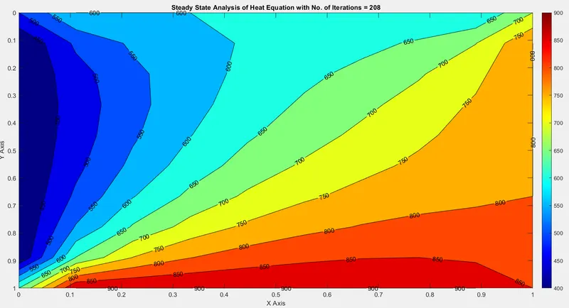
Comments:
- The total number of iterations taken by the solver is 208.
Unsteady Equation Solving using Explicit scheme:
The Unsteady State or Transient state heat conduction is expressed as:
`(delT)/(delt) = alpha((del^2T)/(delx^2) + (del^2T)/(dely^2))`
where,
`(delT)/(delt) -> text(Time domain of the temperature.)`
`(del^2T)/(delx^2) + (del^2T)/(dely^2) -> text(Space domain of Temperature)`
Discretizing the above equation for the unsteady state in explicit scheme using Forward differencing and Central Differencing:
`(T_P^(n+1) - T_P^n)/(nablat) = alpha.((T_L -2T_P +T_R)/(nablax^2) + (T_T - 2T_P + T_B)/(nablay^2))^n`
`T_P^(n+1) = T_P^n + K_1*(T_L-2T_P +T_R)^n+K_2*(T_T-2T_P+T_B)^n`
where,
`K_1 -> alpha.(nablat)/(nablax^2)` and `K_2 -> alpha.(nablat)/(nablay^2)`
Also,
`CFL_x = K_1 and CFL_y = K_2`
Now solving the unsteady state or transient state equation using explicit scheme in MATLAB:
clear all
close all
clc

%Solving the 2D Heat Conduction Equation for Unsteady State
% d2T/dt = alpha*(d2T/dx2 + d2T/dy2)
% Initial and Boundary Condition
% Temperatures,
% Top = 600K, Bottom = 900K, Left = 400K, Right = 800K
t_top = 600;
t_bottom = 900;
t_left = 400;
t_right = 800;
nx = 10;
ny = 10;
T = 298*ones(nx,ny);
T(1,:) = 600; % Top Boundary
T(:,end) = 800; % Right Boundary
T(:,1) = 400; % Left Boundary
T(end,:) = 900; % Bottom Boundary
T(1,1) = 0.5*(t_top + t_left); % Top Left Corner Temperature
T(1,end) = 0.5*(t_top + t_right); % Top Right Corner Temperature
T(end,1) = 0.5*(t_bottom + t_left); % Bottom Left Corner Temperature
T(end,end) = 0.5*(t_bottom + t_right); % Bottom Right Corner Temperature
dx = linspace(0,1,nx);
deltax = dx(2) - dx(1);
dy = linspace(0,1,ny);
deltay = deltax;
deltat = 2e-4;
T_old = T;
alpha = 1.5;
tol = 1e-4;
error = 9e9;
%% Solving the 2D Heat Conduction equation for Unsteady state for explicit solution
k1 = alpha*deltat/deltax^2;
k2 = alpha*deltat/deltay^2;
iter = 1;
for nt = 1:1400 % Time Loop
    while error > tol % Convergance Loop
        for i = 2:nx-1  % Space Loop
            for j = 2:ny-1
                term1 = T_old(i,j);
                term2 = k1*(T_old(i-1,j) - 2*term1 + T_old(i+1,j));
                term3 = k2*(T_old(i,j-1) - 2*term1 + T_old(i,j+1));
                T(i,j) = term1 + term2 + term3;
            end
        end
        iter = iter + 1;
        % Updating the error value
        error = max(max(abs(T_old - T)));
        % Updating the old temperature value
        T_old = T;
        % Plotting the color map
        figure(1)
        contourf(dx,dy,T,'Showtext','on')
        set(gca,'YDir','reverse')
        colormap(jet)
        colorbar
        xlabel('X Axis')
        ylabel('Y Axis')
        title_text = sprintf('Unsteady State Analysis of Heat Equation for Explicit scheme with No. of Iterations = %d',iter);
        title(title_text)
        pause(0.03)
    end
end
Explanation:
- All the input parameters are declared initially which includes boundry conditions, temperature matrix, x and y axis of length 1 m which is descretized with 10 no. of points, error and tolerance value.
- The values for `nablat,nablax and nablay` are assigned.
- After that the value of `K_1 and K_2` is formulated as derived above.
- After declaring all the inputs and constants the solution of the equation will begin with the converging loop which is going to run until the maximum value of the temperature will reach upto a tolerance value of 1e-4.
- The space loop will be started afterwards which calculates the temperature of our domain according to the equation of the steady state heat conduction.
- The whole process is going under the time loop from time steps 1 to 1400.
- At last the results are plotted.
Results:
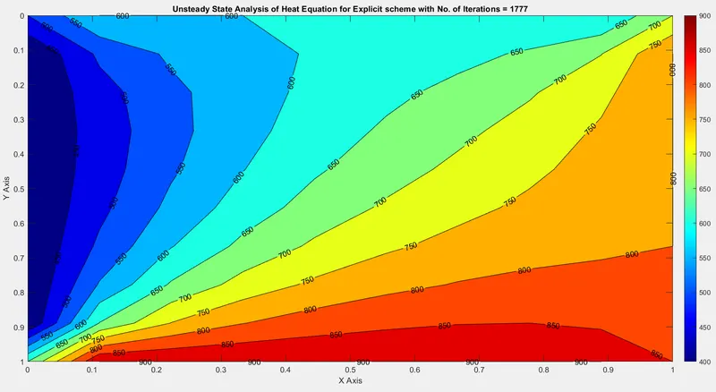
Comments:
- The Number of iterations taken by the Explicit scheme for transient state solver comes out to be 1777.
Unsteady Equation Solving using Implicit scheme:
For Implicit scheme, the Unsteady state equation or transient state equation is given by the expression in descretized form:
`(T_P^(n+1) - T_P^n)/(nablat) = alpha.((T_L -2T_P +T_R)/(nablax^2) + (T_T - 2T_P + T_B)/(nablay^2))^(n+1)`
`T_P^(n+1) = 1/(1 + 2K_1 + 2K_2)(T_P^n + K_1*(T_L+T_R)^(n+1) + K_2*(T_T +T_B)^(n+1))`
The implicit solution of the heat conduction equation is carried out by the iterative solvers. There are 3 types of iterative solvers which we are going to use to solve the implicit solution of the unsteady heat conduction equation.
1. Jacobi Method:
`T_P^(n+1) = 1/(1 + 2K_1 + 2K_2)(T_P^n + K_1*(T_L+T_R)^(n) + K_2*(T_T +T_B)^(n))`
2. Gauss Seidel Method:
`T_P^(n+1) = 1/(1 + 2K_1 + 2K_2)(T_P^n + K_1*(T_L+T_R)^(n+1) + K_2*(T_T +T_B)^(n+1))`
3. Successive Over Relaxation:
`T_P^(n+1) =T_P^n(1-omega) + omega*( 1/(1 + 2K_1 + 2K_2)(T_P^n + K_1*(T_L+T_R)^(n+1) + K_2*(T_T +T_B)^(n+1)))`
Now solving the transient state equation using implicit scheme in MATLAB:
clear all
close all
clc

%% Solving 2D Heat Conduction equation for Unsteady state using Implicit Scheme
% d2T/dt = alpha*(d2T/dx2 + d2T/dy2)
% Initial and Boundary Condition
% Temperatures,
% Top = 600K, Bottom = 900K, Left = 400K, Right = 800K
t_top = 600;
t_bottom = 900;
t_left = 400;
t_right = 800;
nx = 10;
ny = 10;
T = 298*ones(nx,ny); % Initial Temperature = 298K
T(1,:) = 600; % Top Boundary Temperature
T(:,end) = 800; % Right Boundary Temperature
T(:,1) = 400; % Left Boundary Temperature
T(end,:) = 900; % Bottom Boundary Temperature
T(1,1) = 0.5*(t_top + t_left); % Top Left Corner Temperature
T(1,end) = 0.5*(t_top + t_right); % Top Right Corner Temperature
T(end,1) = 0.5*(t_bottom + t_left); % Bottom Left Corner Temperature
T(end,end) = 0.5*(t_bottom + t_right); % Bottom Right Corner Temperature
dx = linspace(0,1,nx);
deltax = dx(2) - dx(1);
dy = linspace(0,1,ny);
deltay = deltax;
deltat = 0.2;
alpha = 1.5;
tol = 1e-4;
error = 9e9;
T_old = T;
T_previous = T_old;
k1 = alpha*deltat/deltax^2;
k2 = alpha*deltat/deltay^2;
CFL = k1 + k2;
w = 1.1; % Relaxation factor
iterative_method = 1; % 1 for Jacobi, 2 for Gauss Seidel and 3 for SOR
%%Jacobi Method
iter = 1;
if iterative_method == 1
    for nt = 1:1400
        while error > tol
            for i = 2:nx-1
                for j = 2:ny-1
                    term1 = (1 + (2*k1) + (2*k2))^-1;
                    term2 = k1*term1;
                    term3 = k2*term1;
                    H = (T_old(i-1,j) + T_old(i+1,j));
                    V = (T_old(i,j-1) + T_old(i,j+1));
                    T(i,j) = (term1*T_previous(i,j)) + (term2*H) + (term3*V);
                end
            end
            iter = iter + 1;
            error = max(max(abs(T_old - T)));
            T_old = T;
        end
        T_previous = T_old;
    end
    figure(1)
    contourf(dx,dy,T,'Showtext','on')
    set(gca,'YDir','reverse')
    colormap(jet)
    colorbar
    xlabel('X Axis')
    ylabel('Y Axis')
    title_text = sprintf('Jacobi Method with %d interations taking %d time steps',iter,nt);
    title(title_text)
    pause(0.03)
end
%% Gauss-Seidel Method
if iterative_method == 2
    for nt = 1:1400
        while error > tol
            for i = 2:nx-1
                for j = 2:ny-1
                    term1 = (1 + (2*k1) + (2*k2))^-1;
                    term2 = k1*term1;
                    term3 = k2*term1;
                    H = (T(i-1,j) + T(i+1,j));
                    V = (T(i,j-1) + T(i,j+1));
                    T(i,j) = (term1*T_previous(i,j)) + (term2*H) + (term3*V);
                end
            end
            iter = iter + 1;
            error = max(max(abs(T_old - T)));
            T_old = T;
        end
        T_previous = T_old;
    end
    figure(2)
    contourf(dx,dy,T,'Showtext','on')
    set(gca,'YDir','reverse')
    colormap(jet)
    colorbar
    xlabel('X Axis')
    ylabel('Y Axis')
    title_text = sprintf('Gauss Seidel Method with %d interations taking %d time steps',iter,nt);
    title(title_text)
    pause(0.03)
end
%% Successive Over Relaxation (SOR) Method
if iterative_method == 3
    for nt = 1:1400
        while error > tol
            for i = 2:nx-1
                for j = 2:ny-1
                    term1 = (1 + (2*k1) + (2*k2))^-1;
                    term2 = k1*term1;
                    term3 = k2*term1;
                    H = (T(i-1,j) + T(i+1,j));
                    V = (T(i,j-1) + T(i,j+1));
                    T(i,j) = (1-w)*T(i,j) + w*((term1*T_previous(i,j)) + (term2*H) + (term3*V));
                end
            end
            iter = iter + 1;
            error = max(max(abs(T_old - T)));
            T_old = T;
        end
        T_previous = T_old;
    end
    figure(3)
    contourf(dx,dy,T,'Showtext','on')
    set(gca,'YDir','reverse')
    colormap(jet)
    colorbar
    xlabel('X Axis')
    ylabel('Y Axis')
    title_text = sprintf('SOR with %d interations taking %d time steps',iter,nt);
    title(title_text)
    pause(0.03)
end
Explanation:
- All the input parameters are declared initially which includes boundry conditions, temperature matrix, x and y axis of length 1 m which is descretized with 10 no. of points, error and tolerance value.
- The values for `nablat,nablax and nablay` are assigned.
- After that the value of `K_1 and K_2` is formulated as derived above.
- A variable called iterative_method is assigned which is used to select the type of iterative solver for our calculations.
- The whole precess is run under the if statement where the variable iterative_method is used to select the type of the iterative solver and calculate the results accordingly.
- After implementing the if statement the solution of the equation will begin with the converging loop which is going to run until the maximum value of the temperature will reach upto a tolerance value of 1e-4.
- The space loop will be started afterwards which calculates the temperature of our domain according to the equation of the steady state heat conduction.
- The whole process is going under the time loop from time steps 1 to 1400.
- At last the results are plotted.
Results:
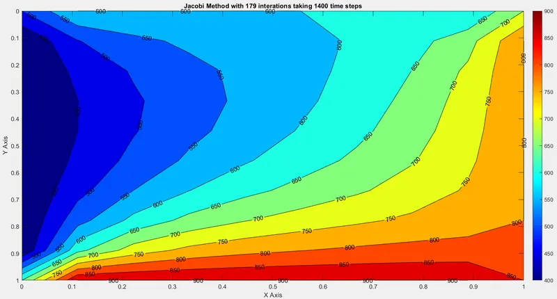
For Jacobi Method:
For Gauss-Seidel Method:
For Successive Over Relaxation (SOR) Method:
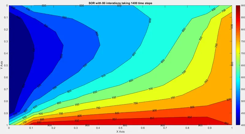
Comments:
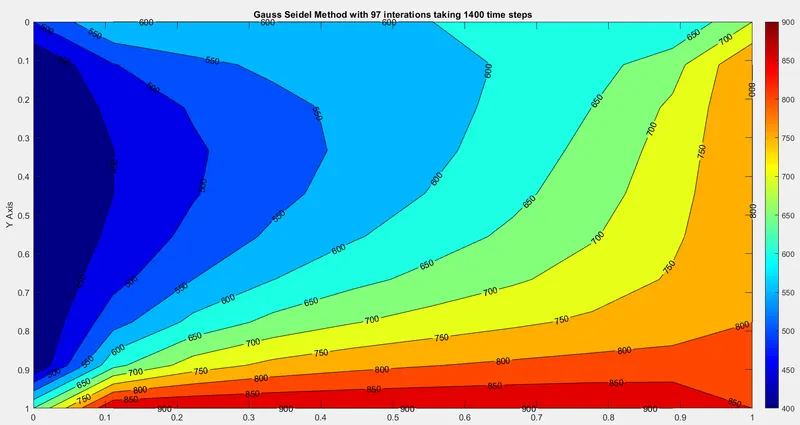
From the above results it is clear that the time taken by the Jacobi method is the longest as it took more number of iterations to complete following the Gauss Seidel method is the second longest time taker and SOR method is third longest.
`text(Jacobi Method > Gauss Seidel Method > SOR)`
Conclusion:
- The 2D heat conduction equation is solved in MATLAB using iterative techniques for implicit scheme.
- The Steady state equation is solved and completed after 208 iterations.
- The Unsteady State Equation under explicit scheme took took longest time with 1777 number of interations performed.
- Out of Jacobi,Gauss Seidel and SOR solvers, the SOR is the fastest running solver to calculate the heat conduction equation.