Simulation of a 1D Super-sonic nozzle flow simulation using MacCormack Method

Aim: To simulate the 1D Super-sonic nozzle flow using MacCormack's technique.

Objective:

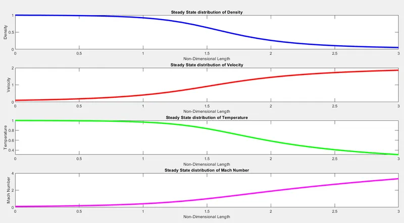
• To show the steady-state distribution of primitive variables inside the nozzle.
• To show the variation of Mass flow rate distribution inside the nozzle at different time steps during the time-marching process for both conservation and non conservation form.
• To compare the normalised mass flow rate distributions of both conservation and non conservation form.

Quasi 1-D Nozzle flow:

The nozzle in which the flow analysis is going to be carried out is shown below.

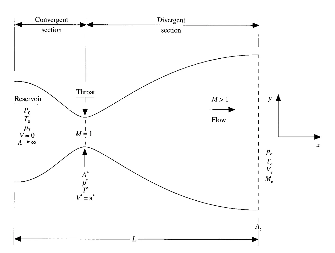
We will consider the steady and isentropic flow through the convergent-divergent nozzle.

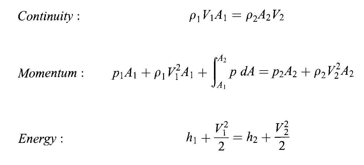
The governing equations for this quasi 1D nozzle flow is expressed as:

Procedure:

We are going to follow the steps listed below to perform the simulation of the supersonic quasi 1D nozzle.

• Creating the mesh in 1-D.
• Discretization.
• Solving.

1. Creating the mesh in 1-D:

The first step involves generating the 1D mesh in the nozzle on x axis as we have assumed that the flow changes only in the x-direction hence the name quasi 1D flow.

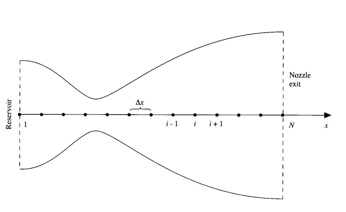
The length of the nozzle is 3 m.

The number of grid points are 31.

2. Dicretization:

The discretization method is done by the MacCormack's technique in this case. MacCormack technique is a kind of predictor-corrector technique which sets up the finite difference expressions. This technique numerically solves the partial differential form of the governing equations using predictor-corrector method where predictor method uses the forward differencing and corrector uses the backward differencing.

The MacCormack's technique is implemented in the following steps:

• Initialisation of the Variables.

In the first step the initial value of the primary variables density, Velocity, temperature and Area of the nozzle must be initialised to proceed the predictor-corrector method.

• Predictor Method.

In this step forward differencing is applied on the target function which in this case are density, velocity, and temperature.

`((delf)/(delt))_p = (f_(i+1) - f_i)/(nablat)`

• Solution Update.

After predicting the values the solution is updated for the target function.

`f_p = f_(text(Initial)) + ((delf)/(delt))_p*nablat`

`f_p-> text(Flow Variables value after the predictor step)`

`f_(Initial)-> text(Initial value of the flow field variables)`

`nablat-> text(Time Step Size)`

• Corrector Method.

In this step backward differencing is applied on the target predicted variables which in this case are density, velocity, and temperature.

`((delf)/(delt))_c = (f_i - f_(i-1))/(nablat)`

After correcting the variables the average of the predicted and corrected value is taken as the final solution of the function.

`(delf)/(delt) = 0.5*(((delf)/(delt))_p + ((delf)/(delt))_c)`

• Final Solution Update.

`f_(sol) = f_(Initial) + (delf)/(delt) *nablat`

`f_(sol) = text(Final solution of the function)`

3. Solving:

This process is done for both conservation and non-conservation form of the governing equation.

Non-Conservative Form:

All the equations are written in non-dimensional form.

(i). Continuity Equation:

In discretized form:

(ii). Momentum Equation:

In discretized form:

(iii). Energy Equation:

In discretized form:

where,

`T' = T/T_0`

`rho' = rho/rho_0`

`x' = x/L`

Denoting the speed of the sound as `a_0`,where

`V' = V/a_0`

`t' =t/(L/a_0)`

`A' = A/A^(**)`

Conservation Form;

All the equations are written in non-dimensional form.

(i). Continuity Equation;

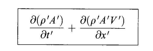= 0

(ii). Momentum Equation;

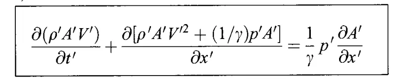
(iii). Energy Equation:

Now implementing the above procedure in MATLAB to solve the equations for the nozzle.

MATLAB function for non-conservation form:

function [rho,V,T,p,dt,iter,net_mfr,mach,mfr,rho_throat,T_throat,p_throat,mach_throat] = non_conservation(n,x,dx,c,nt,gamma,throat)
% Initial Conditions at t = 0
rho = 1 - 0.3146*x; %Density
T = 1 - 0.2314*x; % Temperature
V = (0.1 + 1.09*x).*T.^(1/2); % Velocity
A = 1 + 2.2*(x-1.5).^2; % Area
% Error 
error_rho = 1e9;
error_V = 1e9;
error_T = 1e9;
tol = 1e-5;

iter = 1;
% Outer Time Loop
for k = 1:nt
    rho_old  = rho;
    V_old = V;
    T_old = T;
    %Time Step calculation
    dt = min(c.*(dx./(T.^0.5 + V)));
    if (error_rho > tol && error_V > tol && error_T > tol)
        % Predictor Method
        for j = 2:n-1
            %drho_dt_p = -rho(j)*((V(j+1)-V(j))/dx) - rho(j)*V(j)*((log(A(j+1))-log(A(j)))/dx) - V(j)*((rho(j+1)-rho(j))/dx);
            dV_dx = (V(j+1)-V(j))/dx;
            dlogA_dx = (log(A(j+1))-log(A(j)))/dx;
            drho_dx = (rho(j+1)-rho(j))/dx;
            dT_dx = (T(j+1)-T(j))/dx;
            % Continuity Equation
            drho_dt_p(j) = -rho(j)*dV_dx - rho(j)*V(j)*dlogA_dx - V(j)*drho_dx;
            % Momentum Equation
            dV_dt_p(j) = -V(j)*dV_dx - (1/gamma)*(dT_dx + (T(j)/rho(j))*drho_dx);
            % Energy Equation
            dT_dt_p(j) = -V(j)*dT_dx - (gamma-1)*T(j)*(dV_dx + V(j)*dlogA_dx);
            % Updating the Solution
            rho(j) = rho(j) + drho_dt_p(j)*dt;
            V(j) = V(j) + dV_dt_p(j)*dt;
            T(j) = T(j) + dT_dt_p(j)*dt;

        end
            % Corrector Method
        for j = 2:n-1
            dV_dx = (V(j)-V(j-1))/dx;
            dlogA_dx = (log(A(j))-log(A(j-1)))/dx;
            drho_dx = (rho(j)-rho(j-1))/dx;
            dT_dx = (T(j)-T(j-1))/dx;
            % Continuity Equation
            drho_dt_c(j) = -rho(j)*dV_dx - rho(j)*V(j)*dlogA_dx - V(j)*drho_dx;
            % Momentum Equation
            dV_dt_c(j) = -V(j)*dV_dx - (1/gamma)*(dT_dx + (T(j)/rho(j))*drho_dx);
            % Energy Equation
            dT_dt_c(j) = -V(j)*dT_dx - (gamma-1)*T(j)*(dV_dx + V(j)*dlogA_dx);
        end

        % Averaging the Primary Solution
        drho_dt = 0.5*(drho_dt_p + drho_dt_c);
        dV_dt = 0.5*(dV_dt_p + dV_dt_c);
        dT_dt = 0.5*(dT_dt_p + dT_dt_c);

        % Correction Using the Average Quantities
        for i = 2:n-1
            rho(i) = rho_old(i) + drho_dt(i)*dt;
            V(i) = V_old(i) + dV_dt(i)*dt;
            T(i) = T_old(i) + dT_dt(i)*dt;

        end
        % Applying the Boundary Conditions in Inlet and Outlet
        % Inlet
        V(1) = 2*V(2) - V(3);
        rho(1) = 1;
        T(1) = 1;
        % Outlet
        V(n) = 2*V(n-1) - V(n-2);
        rho(n) = 2*rho(n-1) - rho(n-2);
        T(n) = 2*T(n-1) - T(n-2);
        % Mach Number
        mach = V./sqrt(T);
        % Calculating the mass flow rate
        mfr_in = rho(1)*A(1)*V(1); % Mass Flow Rate at the inlet
        mfr_out = rho(n)*A(n)*V(n); % Mass Flow Rate at the Outlet
        net_mfr(k) = mfr_in - mfr_out;
        
        % Non-Dimensional Variable
        p = rho.*T; % Pressure
        % Mass flow rate at each grid points
        mfr = rho.*A.*V;
        % Calculation of variables at throat of the nozzle
        rho_throat(k) = rho(throat);
        T_throat(k) = T(throat);
        p_throat(k) = p(throat);
        mach_throat(k) = mach(throat);
        % Updating the error
        error_rho = max(abs(rho-rho_old));
        error_V = max(abs(V-V_old));
        error_T = max(abs(T-T_old));
        iter = iter + 1;
        
    end
   % Plotting the Variation in mass flow rate at different time steps
   figure(3)
   hold on
   if k == 50
       plot(x,mfr,'b','linewidth',3)
   elseif k == 100
       plot(x,mfr,'r','linewidth',3)
   elseif k == 150
       plot(x,mfr,'y','linewidth',3)
   elseif k == 200
       plot(x,mfr,'g','linewidth',3)
   elseif k == 700
       plot(x,mfr,'m','linewidth',3)
   end
   xlabel('Non Domensional Distance through nozzle x')
   ylabel('Nondimensional Mass Flow (rho_V_A/rho0_a0_A*)')
   title(' Variation of Mass flow rate distribution inside the nozzle at different time steps during the time-marching process(Non-Conservation form)')
   legend('50dt','100dt','150dt','200dt','700dt')
       
end
end

MATLAB function for conservation form:

function [rho,V,T,p,dt,iter,mach,mfr,rho_throat,T_throat,p_throat,mach_throat] = conservation(n,x,dx,c,nt,gamma,throat)
% Initialization of the primitive variables
for i = 1:n
    if (x(i)>=0 && x(i)<= 0.5)
        rho(i) = 1;
        T(i) = 1;
    elseif (x(i) >= 0.5 && x(i) <= 1.5)
        rho(i) = 1 - 0.366*(x(i) - 0.5);
        T(i) = 1 - 0.167*(x(i) - 0.5);
    elseif (x(i)>= 1.5 && x(i)<= 3.5)
        rho(i) = 0.634 - 0.3879*(x(i) - 1.5);
        T(i) = 0.833 - 0.3507*(x(i) - 1.5);
    end
end

A = 1 + 2.2.*((x-1.5).^2); % Area
V = 0.59./(rho.*A); % Velocity
p = rho.*T; % Pressure
% Time Step Calculation
dt = min(c.*(dx./(T.^0.5 + V)));
iter = 1;
% Solution Vector
U1 = rho.*A;
U2 = U1.*V;
U3 = U1.*((T./(gamma - 1)) + (gamma/2)*V.^2);


% Outer Time loop
for k = 1:nt
    U1_old = U1;
    U2_old = U2;
    U3_old = U3;
    
    % Pure form of Flux terms
    F1 = U2;
    F2 = ((U2.^2)./U1) + ((gamma-1)/gamma)*(U3 - (gamma/2)*((U2.^2)./U1));
    F3 = ((gamma*U2.*U3)./U1) - (gamma*(gamma-1)/2 * ((U2.^3)./U1.^2));
    % Predictor Method
    for j = 2:n-1
        % Source term
        dAdx = ((A(j+1) - A(j))/dx);
        J1(j) = (1/gamma)*rho(j)*T(j)*dAdx;
        % Continuity Equation
        dU1dt_p(j) = -(F1(j+1) - F1(j))/dx;
        % Momentum Equation
        dU2dt_p(j) = -((F2(j+1) - F2(j))/dx) + J1(j);
        % Energy Equation
        dU3dt_p(j) = -(F3(j+1) - F3(j))/dx;

        % Predicted values updated
        U1(j) = U1(j) + dU1dt_p(j)*dt;
        U2(j) = U2(j) + dU2dt_p(j)*dt;
        U3(j) = U3(j) + dU3dt_p(j)*dt;
        % Primitive variables decoded from U1,U2 & U3
        rho(j) = U1(j)/A(j);
        T(j) = (gamma - 1)*((U3(j)/U1(j)) - gamma*0.5*(U2(j)/U1(j))^2);
        p(j) = rho(j)*T(j);
    end
    
    % Corrector Step
    % Pure form of Flux terms
    F1 = U2;
    F2 = ((U2.^2)./U1) + ((gamma-1)/gamma)*(U3 - (gamma/2)*((U2.^2)./U1));
    F3 = ((gamma*U2.*U3)./U1) - (gamma*(gamma-1)/2 * ((U2.^3)./U1.^2));

    for i = 2:n-1
        % Source term
        J2(i) = (1/gamma)*rho(i)*T(i)*((A(i) - A(i-1))/dx);
        % Continuity Equation
        dU1dt_c(i) = -(F1(i) - F1(i-1))/dx;
        % Momentum Equation
        dU2dt_c(i) = -((F2(i) - F2(i-1))/dx) + J2(i);
        % Energy Equation
        dU3dt_c(i) = -(F3(i) - F3(i-1))/dx;
    end
    % Averaging the predictor and corrector terms
    dU1dt = 0.5*(dU1dt_p + dU1dt_c);
    dU2dt = 0.5*(dU2dt_p + dU2dt_c);
    dU3dt = 0.5*(dU3dt_p + dU3dt_c);

    % Final Corrected Values
    for i = 2:n-1
        U1(i) = U1_old(i) + dU1dt(i)*dt;
        U2(i) = U2_old(i) + dU2dt(i)*dt;
        U3(i) = U3_old(i) + dU3dt(i)*dt;
    end
    % Boundary Conditions
    % At Inlet
    U1(1) = rho(1)*A(1);
    U2(1) = 2*U2(2) - U2(3);
    V(1) = U2(1)/U1(1);
    U3(1) = U1(1)*((T(1)/(gamma-1)) + (gamma/2)*V(1)^2);

    % At Outlet
    U1(n) = 2*U1(n-1) - U1(n-2);
    U2(n) = 2*U2(n-1) - U2(n-2);
    U3(n) = 2*U3(n-1) - U3(n-2);

    % Primitive variables decoded by U1,U2 & U3
    rho = U1./A;
    V = U2./U1;
    T = (gamma-1)*(U3./U1 - (gamma/2)*V.^2);
    p = rho.*T;

    % Mach Number
    mach = V./sqrt(T);
    % Mass Flow rate
    mfr = U2;

    % At Throat
    rho_throat(k) = rho(throat);
    T_throat(k) = T(throat);
    p_throat(k) = p(throat);
    mach_throat(k) = mach(throat);
    iter = iter + 1;
   % Plotting the Variation in mass flow rate at different time steps
   figure(6)
   hold on
   if k == 100
       plot(x,mfr,'b','linewidth',1)
   elseif k == 200
       plot(x,mfr,'r','linewidth',1)
   elseif k == 700
       plot(x,mfr,'y','linewidth',1)
   end
   xlabel('Non Domensional Distance through nozzle x')
   ylabel('Nondimensional Mass Flow (rho.V.A/rho_0.a_0.A*)')
   title(' Variation of Mass flow rate distribution inside the nozzle at different time steps during the time-marching process(Conservation form)')
   legend('100dt','200dt','700dt')
end

end

Explanation:

• Functions are named as non_conservation and conservation with the arguments no. of grid points(n), length of the nozzle(x), distance between grid points(dx), courant number (c), no. of time steps (nt), gamma, and throat respectively.
• In the first step primitive variables are initialized which are Density,Pressure,Temperature and Area.
• The time loop will be started in which the predictor and corrector step is initialized.
• In the predictor step all the governing equations are solved and the predicted values of the primitive variables are updated.
• In the corrector step the governing equations are solved and the values of the primitive variables are corrected.
• The final values of the primitive variables are updated.
• The Boundary conditions are specified.
• The values of the primitive variables are found at the throat of the nozzle.
• The graph for the variation of mass flow rate inside the nozzle at time steps 50,100,150,200,&700 during the time-marching process is plotted.

Main Program:

clear all
close all
clc

%Inputs
n = 31;
l = 3;
x = linspace(0,l,n);
dx = x(2) - x(1);
gamma = 1.4;
c = 0.5; % Courant Number
A = 1 + 2.2*(x-1.5).^2; % Area
throat_nc = find(x==1.5); % Throat at x = 1.5
throat_c = find(A==1);
% Time Steps
nt = 700;

% Solving for the Non-Conservation form
[rho_nc,V_nc,T_nc,p_nc,dt_nc,iter_nc,net_mfr_nc,mach_nc,mfr_nc,rho_throat_nc,T_throat_nc,p_throat_nc,mach_throat_nc] = non_conservation(n,x,dx,c,nt,gamma,throat_nc);

% Solving for the Conservation form
[rho_c,V_c,T_c,p_c,dt_c,iter_c,mach_c,mfr_c,rho_throat_c,T_throat_c,p_throat_c,mach_throat_c] = conservation(n,x,dx,c,nt,gamma,throat_c);
% Plotting the results for Non Conservation form
% Steady State distribution of the primitive variables
figure(1)
title('Non-Conservation form')
subplot(4,1,1)
plot(x,rho_nc,'color','b','linewidth',3)
xlabel('Non-Dimensional Length')
ylabel('Density')
title('Steady State distribution of Density')
subplot(4,1,2)
plot(x,V_nc,'color','r','linewidth',3)
xlabel('Non-Dimensional Length')
ylabel('Velocity')
title('Steady State distribution of Velocity')
subplot(4,1,3)
plot(x,T_nc,'color','g','linewidth',3)
xlabel('Non-Dimensional Length')
ylabel('Temperature')
title('Steady State distribution of Temperature')
subplot(4,1,4)
plot(x,mach_nc,'color','m','linewidth',3)
xlabel('Non-Dimensional Length')
ylabel('Mach Number')
title('Steady State distribution of Mach Number')

% Time-wise variation of the primitive variables
figure(2)
subplot(4,1,1)
plot(rho_throat_nc,'b','linewidth',3)
xlabel('No of Time Steps')
ylabel('rho/rho_0')
title('Time-wise variation of Density ratio')

subplot(4,1,2)
plot(p_throat_nc,'r','linewidth',3)
xlabel('No of Time Steps')
ylabel('p/p_0')
title('Time-wise variation of Pressure ratio')

subplot(4,1,3)
plot(T_throat_nc,'g','linewidth',3)
xlabel('No of Time Steps')
ylabel('T/T_0')
title('Time-wise variation of Temperature ratio')

subplot(4,1,4)
plot(mach_throat_nc,'m','linewidth',3)
xlabel('No of Time Steps')
ylabel('Mach Number')
title('Time-wise variation of Mach number')

% Plotting the results for Conservation form
% Steady State distribution of the primitive variables
figure(4)
title('Conservation Form')
subplot(4,1,1)
plot(x,rho_c,'color','b','linewidth',3)
xlabel('Non-Dimensional Length')
ylabel('Density')
title('Steady State distribution of Density')
subplot(4,1,2)
plot(x,V_c,'color','r','linewidth',3)
xlabel('Non-Dimensional Length')
ylabel('Velocity')
title('Steady State distribution of Velocity')
subplot(4,1,3)
plot(x,T_c,'color','g','linewidth',3)
xlabel('Non-Dimensional Length')
ylabel('Temperature')
title('Steady State distribution of Temperature')
subplot(4,1,4)
plot(x,mach_c,'color','m','linewidth',3)
xlabel('Non-Dimensional Length')
ylabel('Mach Number')
title('Steady State distribution of Mach Number')

% Time-wise variation of the primitive variables
figure(5)
subplot(4,1,1)
plot(rho_throat_c,'b','linewidth',3)
xlabel('No of Time Steps')
ylabel('rho/rho_0')
title('Time-wise variation of Density ratio')

subplot(4,1,2)
plot(p_throat_c,'r','linewidth',3)
xlabel('No of Time Steps')
ylabel('p/p_0')
title('Time-wise variation of Pressure ratio')

subplot(4,1,3)
plot(T_throat_c,'g','linewidth',3)
xlabel('No of Time Steps')
ylabel('T/T_0')
title('Time-wise variation of Temperature ratio')

subplot(4,1,4)
plot(mach_throat_c,'m','linewidth',3)
xlabel('No of Time Steps')
ylabel('Mach Number')
title('Time-wise variation of Mach number')

% Comparing mass flow rates distributions of both forms
figure(7)
plot(x,mfr_nc,'b','linewidth',2)
hold on
plot(x,mfr_c,'r','linewidth',2)
xlabel('x/L')
ylabel('Mass Flow rate')
legend('Non-Conservation','Conservation')
title('Comparing Mass Flow rates of conservation and non conservation forms')

Explanation:

• All the Input values are initiated.
• The functions are called for the conservation and non-conservation form.
• All the necessar plots are generated.

Results:

1.Steady-state distribution of primitive variables inside the nozzle.

For Non-Conservation form:

For Conservation form:

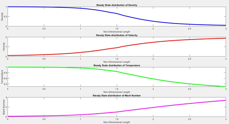
In this steady state distribution plot of both the non-conservation and conservation form we observe the following things:

• The Density and Temperature of both the forms decreases gradually with respect to the x direction and attains minimum value at the outlet of the nozzle.
• The Velocity and Mach number on the other hand increases gradually with respect to the x direction and attains maximum value at the outlet of the nozzle.

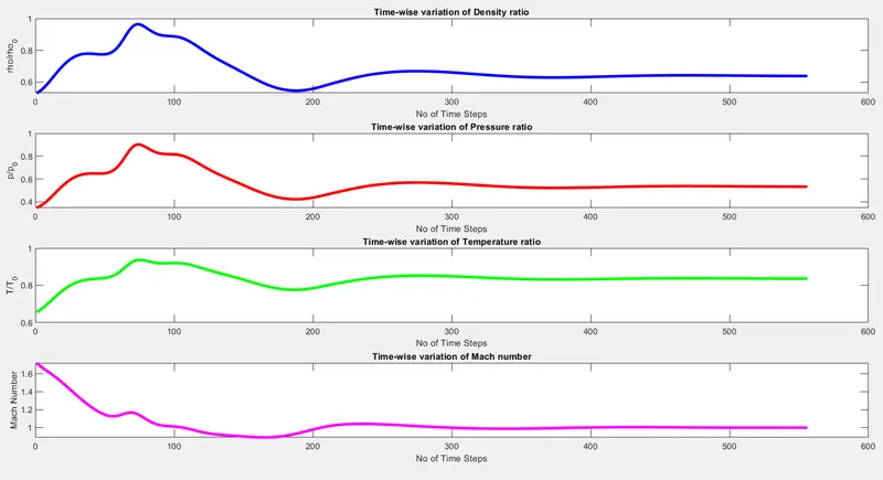
2. Time-wise variation of the primitive variables.

For Non-Conservation form:

For Conservation form:

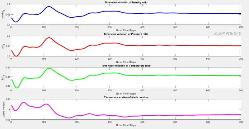
From the above plots for both non-conservative and conservative forms we can observe the following things.

• For the non-conservative plot we can observe that the stability is started to achieve after 200 time steps and after that an exact solution is attained. Also there is not much disturbances in the solution .
• For the conservative plot we observe that it takes much longer to stabilise the solution in conservative form than the nono-conservative form. Also there is alot of disturbances in the solution hence it takes longer iterations than the non-conservative solution.

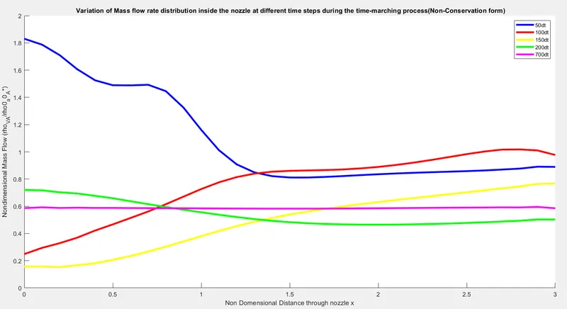
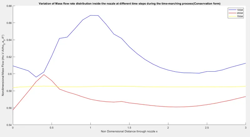
3. Variation of Mass flow rate distribution inside the nozzle at different time steps during the time-marching process.

For Non-Conservative form:

For Conservative form:

• In Non-Conservative form we can observe that in the initial time steps the solution is very unstable , it tries to achieve the stabilty. As the number of time steps increases the disturbances in the graphs tends to lower down which explains that the solution is achivieving the stability gradually and finally at 700 number of time steps the plot is constant straight line ecplained that the solution is stabilised finally.
• In Conservative form there is a lot of disturbances in the initial number of time steps,much higher than that of the non conservative form. That's why conservative form takes much longer time to solve the problem than the non-conservative form.In this case also the the solution is stabilises after the 700 number of time steps.

4. Comparison of Normalized mass flow rate distributions of both forms.

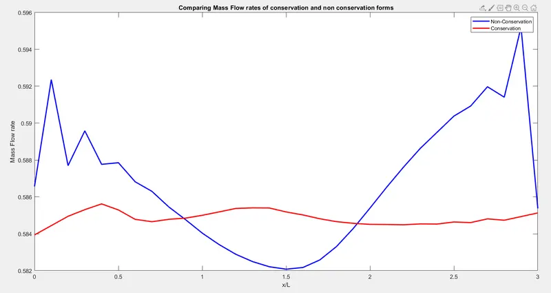
• This plot shows the advantage of conservative form over non-conservative form. The Conservative mass flow is much better than the non-conservative mass flow. So the solution taken by the non-conservative form is faster but the solution of the conservative form is much accurate .

Conclusion:

• The MacCormack's technique is successfully applied on quasi 1D nozzle flow for both the conservative and non conservative form.
• The programs are written along with seperate functions for conservative and non-conservative form.
• All the neccessary plots are shown.
• It has been observed that the non conservati form gives solution faster but conservative form gives the solution much accurately.