Animation of a Simple Pendulum motion Using Python.

Objective: To create a program that solve the following equation:

and then create a simulation of the simple pendulum motion.

Simple Pendulum:

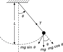
The simple pendulum is another mechanical system that moves in an oscillatory motion. It consists of a point mass ‘m’ suspended by means of light inextensible string of length L from a fixed support. The motion occurs in a vertical plane and is driven by a gravitational force. The forces which are acting on the mass are shown in the figure. The tangential component of the gravitational force, mg sin θ, always acts towards the mean position θ = 0 opposite to the displacement, restoring force acting tangent to the arc.

The motion of the simple pendulum is expressed by the equation:

In the above equation,

g = gravity in m/s2,

L = length of the pendulum in m,

m = mass of the ball in kg,

b=damping coefficient.

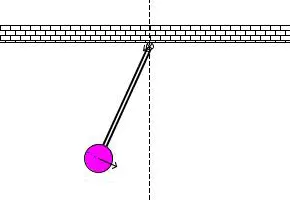
The simulation video is represented as :

To solve the second order differential equation,we need to perform the following process:

we have the second order differential equation:

`(d^2theta)/dt^2 +b/m.(d theta)/dt +g/Lsintheta = 0`

Let's assume,

`theta = theta_1`

So,`(d theta)/dt = (d theta_1)/dt`

Now consider,

`(d theta_1)/dt = theta_2 ........................(1)`

Differntiating on both sides:

`(d^2theta_1)/dt^2 = (d theta_2)/dt`

Put these expressions in the above second order differential equation,

`(d^2theta_1)/dt^2 + b/m.(d theta_1)/dt+g/Lsintheta_1 = 0`

`(d theta_2)/dt + b/m.theta_2 + g/Lsintheta_1 = 0 ........................(2)`

Based on these equations i.e, Eq 1 and 2,we have solution vector:

`(d theta)/dt = [[theta_2],[(d theta_2)/dt = -b/mtheta_2-g/Lsintheta_1]]`

Now we have to make a python program to solve this equation and plot the results:

Given data:

L=1 metre,

m=1 kg,

b=0.05.

g=9.81 m/s2.

Program:

import math
import matplotlib.pyplot as plt
import numpy as np
from scipy.integrate import odeint

def model(theta,time,b,g,l,m):
	theta1 = theta[0]
	theta2 = theta[1]
	dtheta1_dt = theta2
	dtheta2_dt = -(b/m)*theta2 - (g/l)*math.sin(theta1)
	dtheta_dt = [dtheta1_dt,dtheta2_dt]
	return dtheta_dt

b = 0.05
g = 9.81
l = 1
m = 0.1

# initial condition
theta_0 = [0,3]

# time points
time = np.linspace(0,20,300)

# Solving ODE
theta = odeint(model,theta_0,time,args = (b,g,l,m))


Angular_displacement = []
Angular_velocity = []

for j in range(0,len(theta)):
	displacement = theta[j,0]
	Angular_displacement.append(displacement)

	velocity = theta[j,1]
	Angular_velocity.append(velocity)



#Creating a for loop to make arrays of angular displacement and velocity


# plotting the results

plt.figure(1)
plt.plot(time,theta[:,0],'b-',label = r'$frac{dtheta_1}{dt} = theta_2$')
plt.plot(time,theta[:,1],'r--',label = r'$frac{dtheta_2}{dt} = -frac{b}{m}theta_2 - frac{g}{l}sintheta_1$')
plt.xlabel('Time')
plt.ylabel('Plot')
plt.legend(loc = 'best')
plt.show()

# Simulating the simple pendulum
x0 = 0
y0 = 0
# creating a for loop to simulate the simple pendulum
ct = 1
for i in range(0,len(time)):
	THETA = Angular_displacement[i]
	x1 = l*math.sin(THETA)
	y1 = -l*math.cos(THETA)
	filename = 'pendulum%05d' % ct
	ct = ct + 1


	plt.figure(2)
	plt.plot([-1,1],[0,0],color = 'r')
	plt.plot([x0,x1],[y0,y1])
	plt.plot(x1,y1,marker = 'o',markerfacecolor = 'g',markeredgecolor  = 'k',markersize = 15)
	plt.xlim([-2,3])
	plt.ylim([-3,3])
	plt.title('Animation of Simple pendulum motion',fontsize = 20,fontweight = 'bold')
	plt.savefig(filename)
	plt.clf()

Explanation of the codes:

1. All the necessary libraries have been imported.A special library called scipy.integrate is used to solve the second order differential equation.
2. Defining a function named model with the arguments theta,time,b,g,l and m.
3. All the inputs are given.
4. Initial condition have been given to the variable theta_0 as [0,3] which means that the initial position of the pendulum is zero and the initial velocity of the pendulum is 3 rad/s.
5. Specifying the time interval from 0 to 20 sec.
6. Now solving the 2nd order ODE as odeint command written as theta = odeint(model,theta_0,time,args = (b,g,l,m)). In this command the function odeint is used to integrate the equation and in this case dtheta_dt is the solution vector that needs to be solved using this command.
7. Two arrays have been initiated named Angular_displacement and Angular_velocity so that all the values calculated from the odeint function can be stored in these two respective arrays.
8. A for loop is created to the range 0 to theta where two variables displacement and velocity has some value for every value of theta and these values is then appended to the empty arrays Angular_displacement and Angular_velocity respectively.
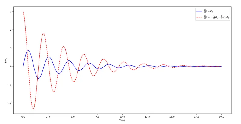
9. Now plotting the plot for this simple harmonic motion versus time.
10. Now we have to animate the motion of the simple pendulum.
11. Entering the inputs of the coordinates.
12. Creating a for loop to capture each and every figure of the simple pendulum position with respect to time.
13. ct is a counter variable that is added to place each and every figure sequence wise.
14. Plotting the result in an folder and store all the figures.
15. marker command is used to create pendulum bob.

Results:

Simulation video: