Validation studies of Symmetry BC vs Wedge BC in OpenFOAM vs Analytical H.P equation
Objective:
- To perform the validation studies of Symmetry BC and wedge BC with the analytical Hagen-Poiseulle's equation.
Expected Results:
- Validate Hydro-dynamic length with the numerical result
- Validate the fully developed flow velocity profile with its analytical profile
- Validate maximum velocity and pressured drop for fully developed flow
- Post-process Shear stress and validate wall shear stress for fully developed flow
- Highlight the differences in both boundary conditions in terms of their usage and aplication
Symmetry Boundary Condition:
The symmetry boundary condition defines a mirror face/surface. It should only be used if the physical object or geometry and the expected flow field pattern of the developed solution are mirrored along that surface. By using this boundary condition, the domain can essentially be halved, reducing the time to achieve a solution.
In detail, the symmetry condition applies the following constraints on the flow variables:
- The fluxes across the symmetry are zero.
- The normal components of all variables are set to zero.
It can be applied to both planar or non-planar faces/surfaces on the domain boundaries.
Wedge Boundary Condition:
The wedge boundary condition (BC) is used in computational fluid dynamics to define an axisymmetric situation, for eg. cylinder. The model and flow must be axisymmetric along a central line such that all physical variables of the flow have the same value and distribution at a given radius for all angles.
This boundary condition is specified by two planes that must be selected on separate sides of the domain (referred to as front and back) on surfaces running along the axis. It works for 2D simulations only.
Wedge is different from the symmetry boundary condition in the sense that the wedge BC applies the Navier-Stokes equations in cylindrical coordinates whereas the latter applies in cartesian coordinates. One big advantage of wedge is that it allows for the rotational flow around the axis and this is possible only because the fluxes and normal components are not assumed as zero.
Hagen-Poiseulle's equation:
In standard fluid-kinetics notation:
- Δ p = 8 μ L Q π R 4 = 8 π μ L Q A 2 {displaystyle Delta p={frac {8mu LQ}{pi R^{4}}}={frac {8pi mu LQ}{A^{2}}}}
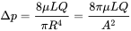
where:
- Δp is the pressure difference between the two ends,
- L is the length of pipe,
- μ is the dynamic viscosity,
- Q is the volumetric flow rate,
- R is the pipe radius,
- A is the cross section of pipe.
The equation does not hold close to the pipe entrance.
The equation fails in the limit of low viscosity, wide and/or short pipe. Low viscosity or a wide pipe may result in turbulent flow, making it necessary to use more complex models, such as the Darcy–Weisbach equation. The ratio of length to radius of a pipe should be greater than one forty-eighth of the Reynolds number for the Hagen–Poiseuille law to be valid. If the pipe is too short, the Hagen–Poiseuille equation may result in unphysically high flow rates; the flow is bounded by Bernoulli's principle, under less restrictive conditions, by
- Δ p = 1 2 ρ v ¯ max 2 = 1 2 ρ ( Q max π R 2 ) 2 → Q max = π R 2 2 Δ p ρ , {displaystyle Delta p={frac {1}{2}}rho {overline {v}}_{text{max}}^{2}={frac {1}{2}}rho left({frac {Q_{max }{}}{pi R^{2}}}right)^{2},,,rightarrow ,,,Q_{max }{}=pi R^{2}{sqrt {frac {2Delta p}{rho }}},}

because it is impossible to have less-than-zero (absolute) pressure (not to be confused with gauge pressure) in an incompressible flow.
The hydrodynamic entrance region refers to the area of a pipe where fluid entering a pipe develops a velocity profile due to viscous forces propagating from the interior wall of a pipe. This region is characterized by a non-uniform flow. The fluid enters a pipe at a uniform velocity, then fluid particles in the layer in contact with the surface of the pipe come to a complete stop due to the no-slip condition. Due to viscous forces within the fluid, the layer in contact with the pipe surface resists the motion of adjacent layers and slows adjacent layers of fluid down gradually, forming a velocity profile. For the conservation of mass to hold true, the velocity of layers of the fluid in the center of the pipe increases to compensate for the reduced velocities of the layers of fluid near the pipe surface. This develops a velocity gradient across the cross section of the pipe.
The length of the hydrodynamic entry region along the pipe is called the hydrodynamic entry length. It is a function of Reynolds number of the flow. In case of laminar flow, this length is given by:
L h , l a m i n a r = 0.05 R e D {displaystyle L_{h,laminar}=0.05R_{e}D} 
The average velocity is calculated as :
`U_(avg) = (R_emu)/(rhoD)`
The velocity variation along the radius is given by:
`U(r) = 2*U_(avg)*(1-(r^2)/R^2)`
where,
r is the variable radius of the pipe.
and R is the maximum radius of the pipe.
The pressure drop along the length of the pipe is analytically calculated as,
`Deltap = (32muLU_(avg))/D^2`
The wall shear stress can be analytically calculated as,
Darcy friction factor, `f = 64/R_e`
`tau_(wall) = f/4*(rhoU_(avg)^2)/2`
1. Simulation for `10^o` angle:
The follwing steps will be follwed while simulating the flow,
- Genertaing the blockMeshDict file for 10 deg.
- Applying suitable boundry conditions.
- Setting up the simulation oarameters and run the simulation.
Case 1: Wedge BC:
(i). Generating blockMeshDict file:
The below is the blockMeshDict file for the wedge boundary condition:
/*--------------------------------*- C++ -*----------------------------------*
  =========                 |
  \      /  F ield         | OpenFOAM: The Open Source CFD Toolbox
   \    /   O peration     | Website:  https://openfoam.org
    \  /    A nd           | Version:  8
     \/     M anipulation  |
*---------------------------------------------------------------------------*/
FoamFile
{
    version     2.0;
   format      ascii;
    class       dictionary;
    object      blockMeshDict;
}
// * * * * * * * * * * * * * * * * * * * * * * * * * * * * * * * * * * * * * //

convertToMeters 1;

vertices
(
    (0 0 0) // Vertex 0
    (0 0.003985 -0.000349) // Vertex 1
    (0 0.003985 0.000349) // Vertex 2
    (2.000000e-01 0 0) // Vertex 3
    (2.000000e-01 0.003985 -0.000349) // Vertex 4
    (2.000000e-01 0.003985 0.000349) // Vertex 5
);
blocks
(
    hex (0 1 2 0 3 4 5 3) (50 1 400) simpleGrading (0.1 1 10)
);

edges
(
   arc 1 2 (0 4.000000e-03 0)
   arc 4 5 (2.000000e-01 4.000000e-03 0)
);

boundary
(
   axis
   {
     type empty;
     faces
     (
            (0 3 3 0)
     );
   }

   inlet
   {
     type patch;
     faces
     (
            (0 0 2 1)
     );
   }

   wall
   {
     type wall;
     faces
     (
            (2 5 4 1)
     );
   }

   outlet
   {
     type patch;
     faces
     (
            (3 4 5 3)
     );
   }

   front
   {
     type wedge;
     faces
     (
            (0 3 5 2)
     );
   }

   back
   {
     type wedge;
     faces
     (
            (0 1 4 3)
     );
   }

);

mergePatchPairs
(
);

// ************************************************************************* //
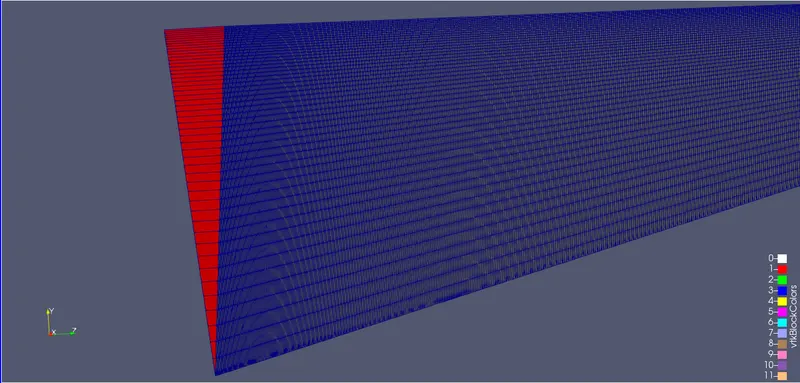
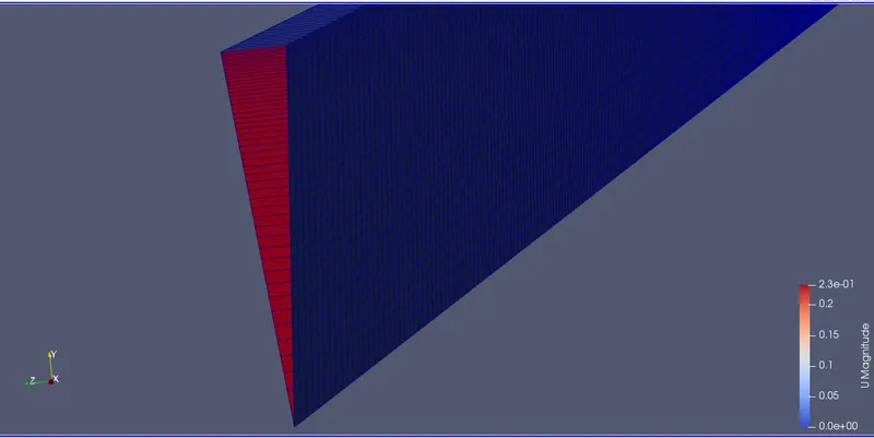
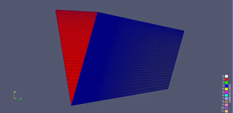
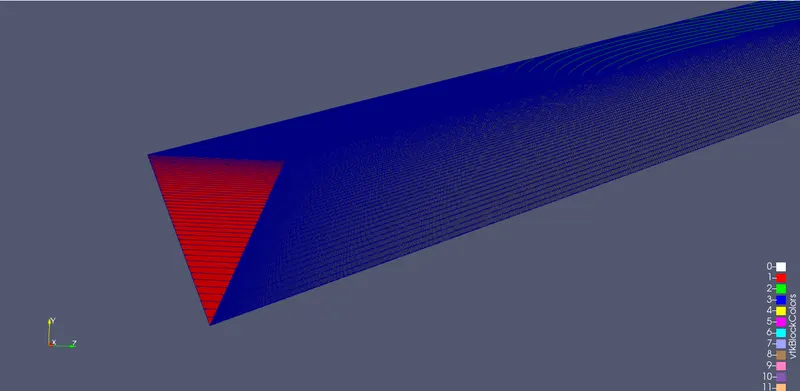
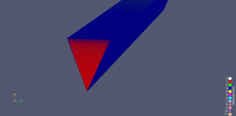
The block after implementing blockMesh command is represented as:
(ii). Applying suitable boundary condition:
controlDict file:
/*--------------------------------*- C++ -*----------------------------------*
  =========                 |
  \      /  F ield         | OpenFOAM: The Open Source CFD Toolbox
   \    /   O peration     | Website:  https://openfoam.org
    \  /    A nd           | Version:  8
     \/     M anipulation  |
*---------------------------------------------------------------------------*/
FoamFile
{
    version     2.0;
    format      ascii;
    class       dictionary;
    location    "system";
    object      controlDict;
}
// * * * * * * * * * * * * * * * * * * * * * * * * * * * * * * * * * * * * * //

application     icoFoam;

startFrom       startTime;

startTime       0;

stopAt          endTime;

endTime         20;

deltaT          0.01;

writeControl    timeStep;

writeInterval   2000;

purgeWrite      0;

writeFormat     ascii;

writePrecision  6;

writeCompression off;

timeFormat      general;

timePrecision   6;

runTimeModifiable true;


// ************************************************************************* //
Velocity boundary condition:
/*--------------------------------*- C++ -*----------------------------------*
  =========                 |
  \      /  F ield         | OpenFOAM: The Open Source CFD Toolbox
   \    /   O peration     | Website:  https://openfoam.org
    \  /    A nd           | Version:  8
     \/     M anipulation  |
*---------------------------------------------------------------------------*/
FoamFile
{
    version     2.0;
    format      ascii;
    class       volVectorField;
    object      U;
}
// * * * * * * * * * * * * * * * * * * * * * * * * * * * * * * * * * * * * * //

dimensions      [0 1 -1 0 0 0 0];

internalField   uniform (0.50929 0 0);

boundaryField
{
    axis
    {
        type            empty;
    }

    inlet
    {
        type            fixedValue;
        value           uniform (0.50929 0 0);
    }

    wall
    {
        type            fixedValue;
        value		 uniform (0 0 0);
    }
    outlet
    {
        type            inletOutlet;
        inletValue      uniform (0.50929 0 0);
        value		 uniform (0.50929 0 0);
    }
    front
    {
        type            wedge;
    }
    back
    {
        type            wedge;
    }
}

// ************************************************************************* //
Pressure boundary condition:
/*--------------------------------*- C++ -*----------------------------------*
  =========                 |
  \      /  F ield         | OpenFOAM: The Open Source CFD Toolbox
   \    /   O peration     | Website:  https://openfoam.org
    \  /    A nd           | Version:  8
     \/     M anipulation  |
*---------------------------------------------------------------------------*/
FoamFile
{
    version     2.0;
    format      ascii;
    class       volScalarField;
    object      p;
}
// * * * * * * * * * * * * * * * * * * * * * * * * * * * * * * * * * * * * * //

dimensions      [0 2 -2 0 0 0 0];

internalField   uniform 0;

boundaryField
{
    axis
    {
        type            empty;
    }

    inlet
    {
        type            zeroGradient;
    }

    wall
    {
        type            zeroGradient;
    }
    outlet
    {
        type            fixedValue;
        value		 uniform 10;
    }
    front
    {
        type            wedge;
    }
    back
    {
        type            wedge;
    }
}

// ************************************************************************* //
These files are gonna be same for all the 5 remaining cases except for symmetry boundary conditions the patch types are replaced by symmetry keyword instead of wedge keyword. For example,
   front
   {
     type symmetry;
     faces
     (
            (0 3 5 2)
     );
   }

   back
   {
     type symmetry;
     faces
     (
            (0 1 4 3)
     );
Results:
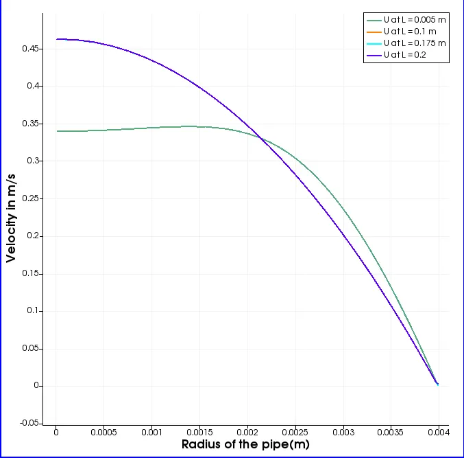
Velocity variation over the radius of the pipe along different locations :
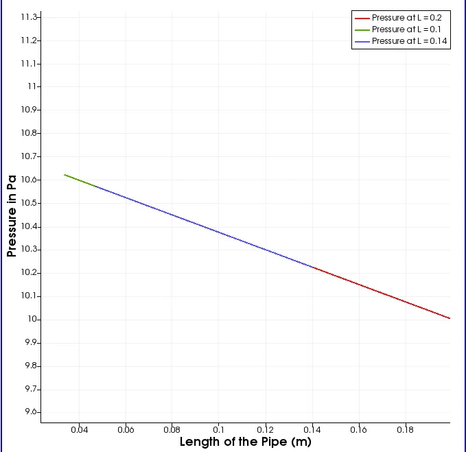
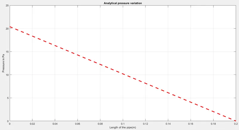
Pressure variation over the length of the pipe:
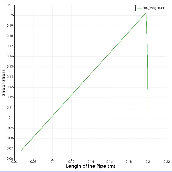
Shear Stress variation over the length of the pipe:
Validating the results using MATLAB:
clear all
close all
clc

% Inputs
Q = 25.6e-6;% Flow rate at inlet
L = 200e-3; % Length of the pipe in mm
Re = 2100; % Reynolds Number
D = 8e-3; % Diameter of the pipe in mm
theta = 10; %angle of the wedge in degrees.
rho = 997; % density in kg/m3.
R = D/2; %Radius of the pipe
mu = 8.8e-4; %Dynamic Viscosity Pa.s
Lh = 0.05*mu*D; % hydro-dynamic entrance length
nx = 50;
ny = 1;
nz = 400;

% Generating blockMEshDict file
file = blockMesh(R,theta,L,nx,ny,nz);

% Analytical Solution
% Average Velocity
U_avg = (Re*mu)/(rho*D);

%Maximum Velocity
U_max = 2*U_avg;

% Velocity Vector
r = linspace(0,R,1001);
U_r = 2*U_avg*(1-((r.^2)/R^2));

%Pressure Vector
l = linspace(0,L,1001);
delta_Pr = (32*mu*l*U_avg)/(D^2);
P_r = fliplr(delta_Pr);
P_r = P_r';

% Wall Shear stress calculation
f = 64/Re;
tau_wall = (f/4)*((rho*U_avg^2)/2);

% Plotting the results for validation
% Plotting Velocity variation Analytical
figure(1)
plot(r,U_r,'--b','linewidth',3)
xlabel('Radius of the pipe(m)')
ylabel('Velocity in m/s')
title('Analytical velocity variation')
grid on

% Pressure variation Analytical
figure(2)
plot(l,P_r,'--r','linewidth',3)
xlabel('Length of the pipe(m)')
ylabel('Pressure in Pa')
title('Analytical pressure variation')
grid on 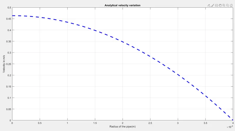
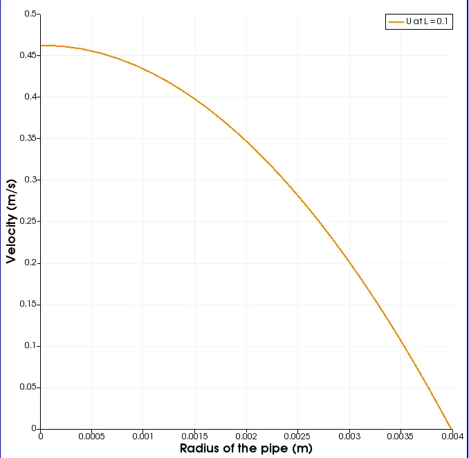
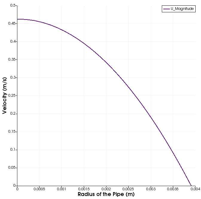
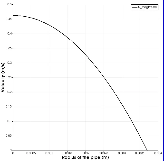
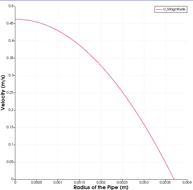
- The Analytical velocity variation graph exactly traces the numerical velocity variation plot.
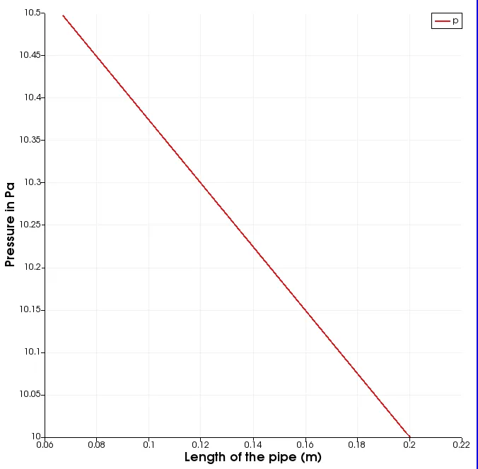
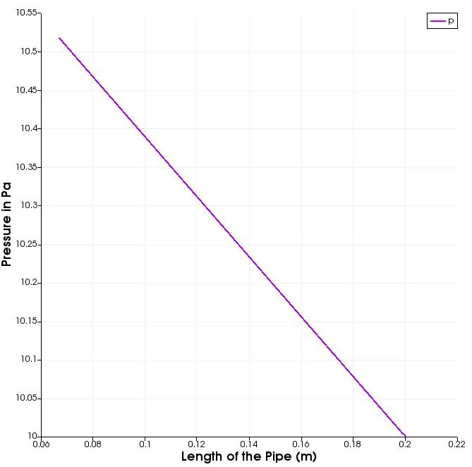
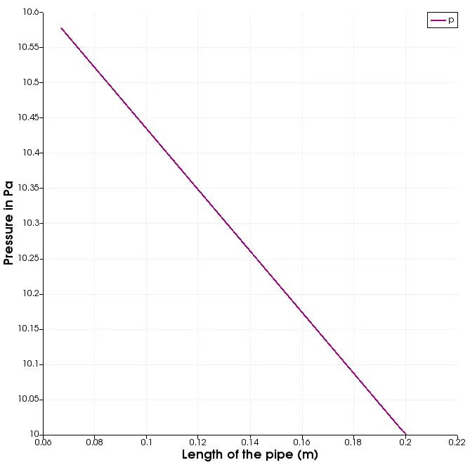
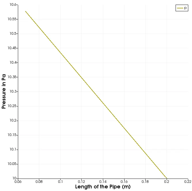
- The Analytical pressure variation plot exactly matches the numerica pressure variation plot.
Now we have 5 more cases to perform namely:
- Wedge BC for angle `25^o`.
- Wedge BC for angle `45^o`.
- Symmetry BC for angle `10^o`.
- Symmery BC for angle `25^o`.
- Symmetry BC for angle `45^o`.
As these cases also follows the same steps as we have showed in the case of wedge BC for `10^o` we will only show the results of these cases.
Case 2: Symmetry BC
Velocity variation over the radius of the pipe along the length of the pipe :
Variation of Pressure field along the length of the pipe:
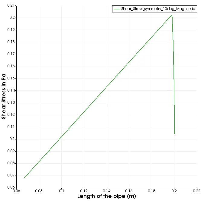
Shear stress variation along the length of the pipe:
Validating the results using MATLAB:
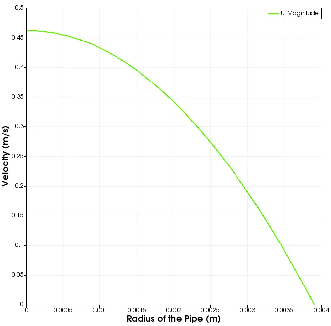
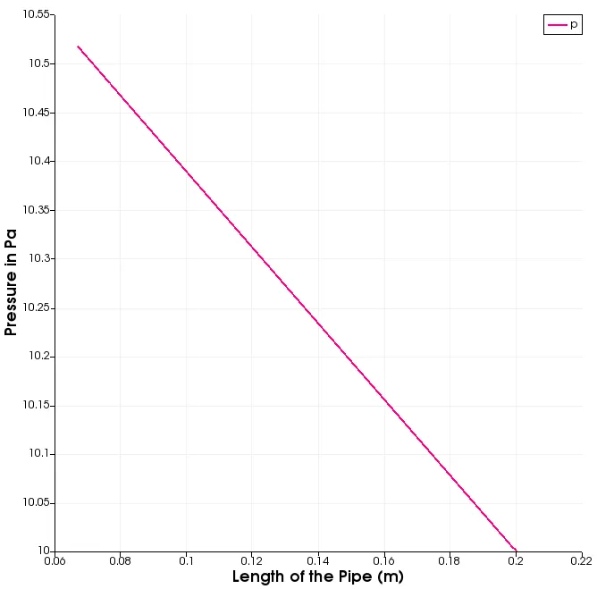
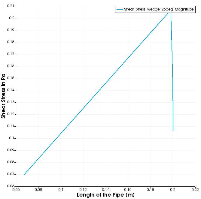
2. Simulation for `25^o` angle:
Case 1: For Wedge Boundary Condition
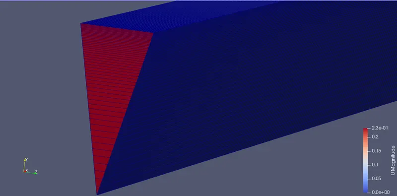
Velocity variation over the radius of the pipe along the length of the pipe :
Variation of Pressure field along the length of the pipe:
Shear stress variation along the length of the pipe:
Case 2: For Symmetry Boundary Condition
Velocity variation over the radius of the pipe along the length of the pipe :
Variation of Pressure field along the length of the pipe:
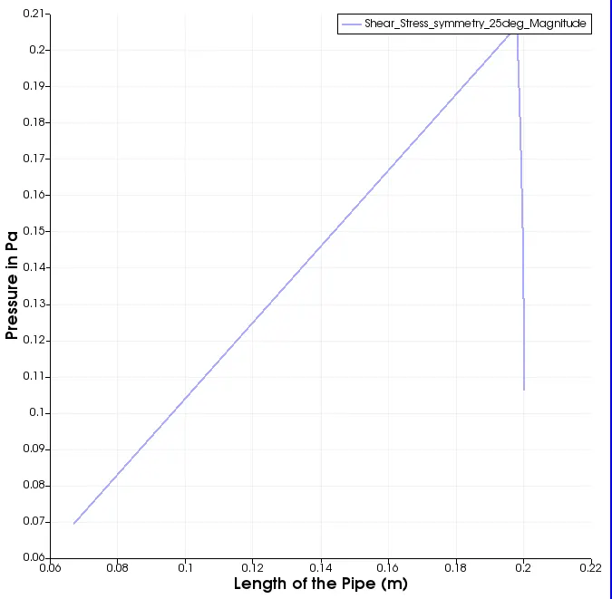
Shear stress variation along the length of the pipe:
Validating the results using MATLAB:
3. Simulation for `45^o` angle:
Case 1: Wedge Boundary Condition:
Velocity variation over the radius of the pipe along the length of the pipe :
Variation of Pressure field along the length of the pipe:
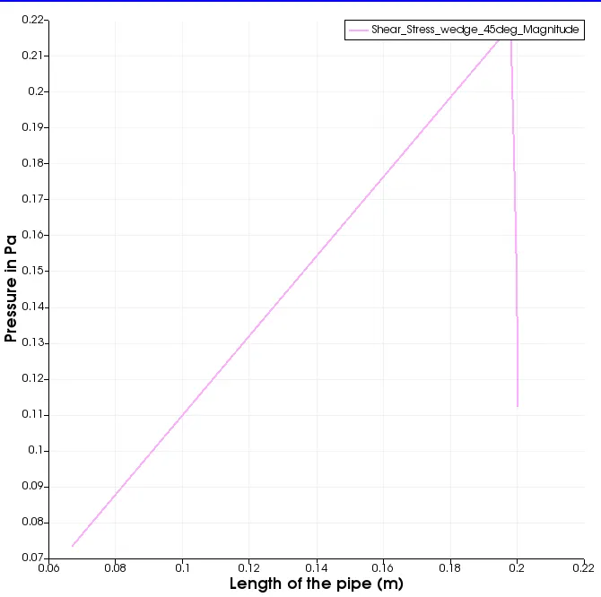
Shear stress variation along the length of the pipe:
Case 2: Symmetry boundary condition:
Velocity variation over the radius of the pipe along the length of the pipe :
Variation of Pressure field along the length of the pipe:
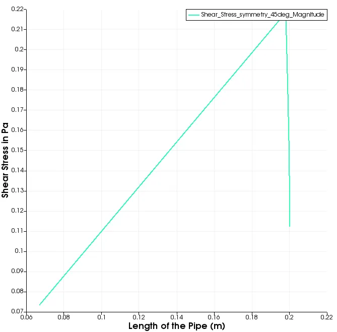
Shear stress variation along the length of the pipe:
Validating the results using MATLAB:
Conclusion:
- Theoritcally the Wedge and Symmetry boundary conditions are different but they produced the exact same solution for different angles of the wedges.
- Analytical solution of the velocity and pressure produced the exact result as with the numerical solution.