Surface defects on Steel plates classification using SVM algorithm
Objective: In this project we will be carrying out the Support Vector Machine (SVM) algorithm to the Steel plates faults dataset and anlysing the accuracy of the model.
Overview:
- Explanation of Support Vector Machine(SVM) algorithm.
- Explaining advantages and disadvantages of SVM algorithm.
- Performing Exploratory Data Analysis (EDA) on the Steel plates defects dataset.
- Implementing Support Vector Machine (SVM) algorithm on the Steel plates defects datasets.
- Summarizing and concluding the observations.
Support Vector Machines (SVM):
“Support Vector Machine” (SVM) is a supervised machine learning algorithm which can be used for both classification or regression challenges. However, it is mostly used in classification problems. In the SVM algorithm, we plot each data item as a point in n-dimensional space (where n is number of features you have) with the value of each feature being the value of a particular coordinate. Then, we perform classification by finding the hyper-plane that differentiates the classes very well.
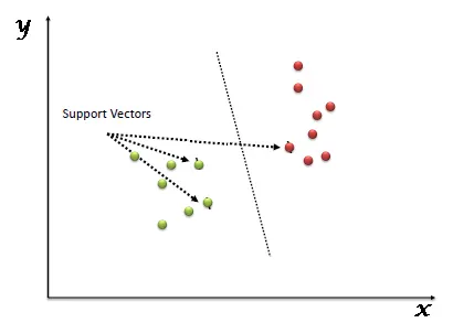
Support Vectors are simply the co-ordinates of individual observation. The SVM classifier is a frontier which best segregates the two classes (hyper-plane/ line).
Let's see how the SVM algorithm works.This involves the following steps to perform the task.
- Identify the right hyper-plane (Scenario-1): Here, we have three hyper-planes (A, B and C). Now, identify the right hyper-plane to classify star and circle.
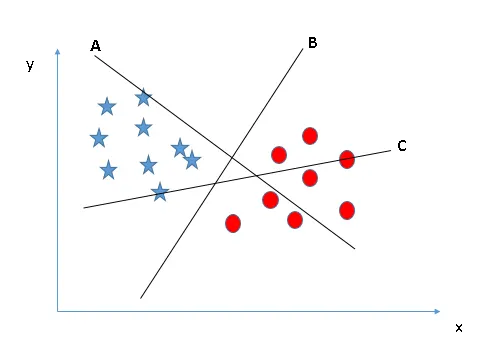
W need to remember a thumb rule to identify the right hyper-plane: “Select the hyper-plane which segregates the two classes better”. In this scenario, hyper-plane “B” has excellently performed this job.
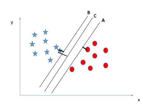
- Identify the right hyper-plane (Scenario-2): Here, we have three hyper-planes (A, B and C) and all are segregating the classes well. Now, How can we identify the right hyper-plane?
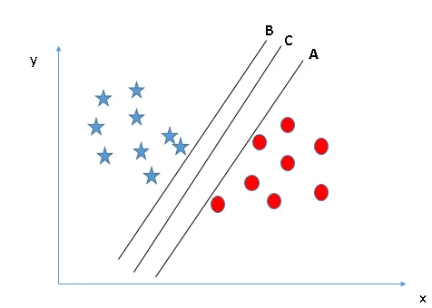 Here, maximizing the distances between nearest data point (either class) and hyper-plane will help us to decide the right hyper-plane. This distance is called as Margin. Let’s look at the below snapshot: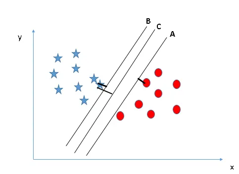
Above, we can see that the margin for hyper-plane C is high as compared to both A and B. Hence, we name the right hyper-plane as C. Another lightning reason for selecting the hyper-plane with higher margin is robustness. If we select a hyper-plane having low margin then there is high chance of miss-classification. - Identify the right hyper-plane (Scenario-3):
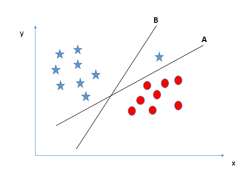 In this case, SVM selects the hyper-plane which classifies the classes accurately prior to maximizing margin. Here, hyper-plane B has a classification error and A has classified all correctly. Therefore, the right hyper-plane is A.
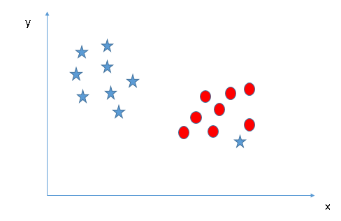
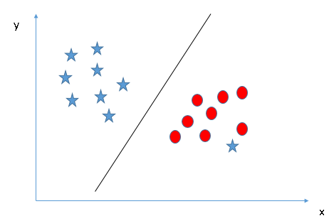
- Can we classify two classes (Scenario-4)?: Below, we are unable to segregate the two classes using a straight line, as one of the stars lies in the territory of other(circle) class as an outlier.
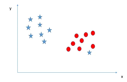 As it is already mentioned, one star at other end is like an outlier for star class. The SVM algorithm has a feature to ignore outliers and find the hyper-plane that has the maximum margin. Hence, we can say, SVM classification is robust to outliers.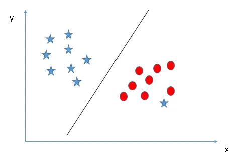
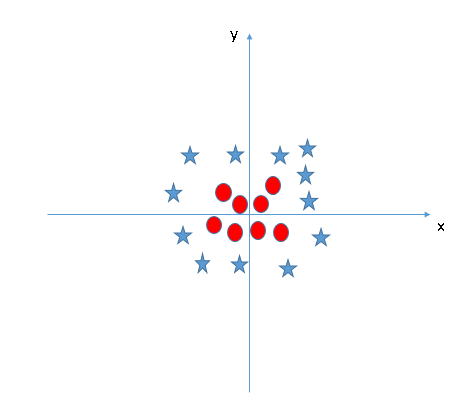
- Find the hyper-plane to segregate to classes (Scenario-5): In the scenario below, we can’t have linear hyper-plane between the two classes, so how does SVM classify these two classes? Till now, we have only looked at the linear hyper-plane.
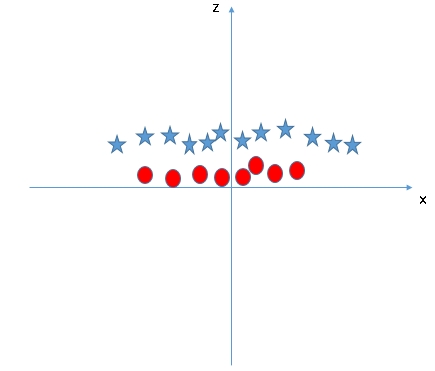
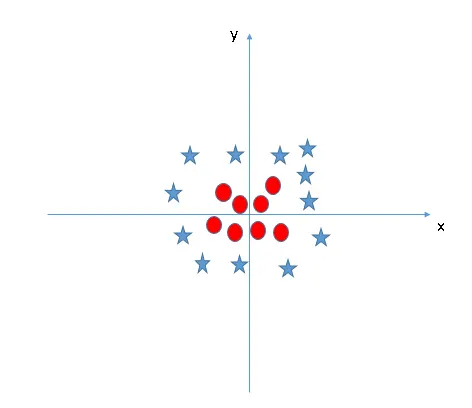 SVM can solve this problem. Easily! It solves this problem by introducing additional feature. Here, we will add a new feature z=x^2+y^2. Now, let’s plot the data points on axis x and z: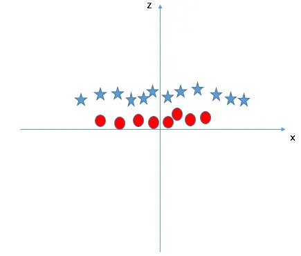
In above plot, points to consider are:- All values for z would be positive always because z is the squared sum of both x and y
- In the original plot, red circles appear close to the origin of x and y axes, leading to lower value of z and star relatively away from the origin result to higher value of z.
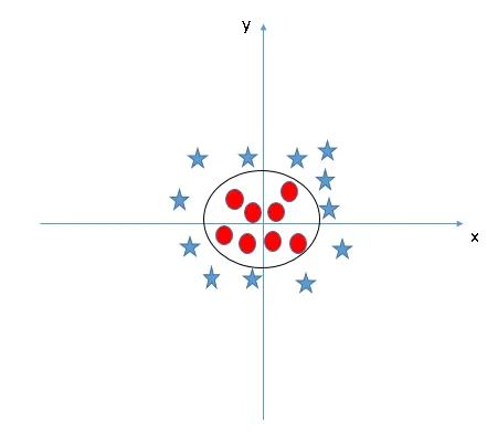
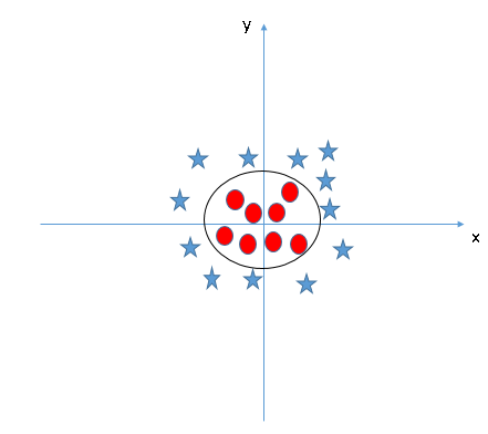
In the SVM classifier, it is easy to have a linear hyper-plane between these two classes. But, another burning question which arises is, should we need to add this feature manually to have a hyper-plane. No, the SVM algorithm has a technique called the kernel trick. The SVM kernel is a function that takes low dimensional input space and transforms it to a higher dimensional space i.e. it converts not separable problem to separable problem. It is mostly useful in non-linear separation problem. Simply put, it does some extremely complex data transformations, then finds out the process to separate the data based on the labels or outputs you’ve defined.
When we look at the hyper-plane in original input space it looks like a circle:
Pros and Cons of SVM :
Pros:
- It works really well with a clear margin of separation
- It is effective in high dimensional spaces.
- It is effective in cases where the number of dimensions is greater than the number of samples.
- It uses a subset of training points in the decision function (called support vectors), so it is also memory efficient.
Cons:
- It doesn’t perform well when we have large data set because the required training time is higher.
- It also doesn’t perform very well, when the data set has more noise i.e. target classes are overlapping
- SVM doesn’t directly provide probability estimates, these are calculated using an expensive five-fold cross-validation. It is included in the related SVC method of Python scikit-learn library.
Performing EDA on the Steel plates defectss dataset:
In this process we are going to import the data of Steel plates defects dataset provided in the question.
The EDA analysis of the dataset will be carried out in the following steps:
- Data preperation and cleaning.
- Data visualisation.
- Finding the correlations between the features.
- Analysing the Feature skewness.
- Analysing the outliers.
- Summary and Conclusion.
1. Data preperation and cleaning:
In this process we will first import the data and check how it looks like .
import numpy as np
import pandas as pd
import seaborn as sns
import matplotlib.pyplot as plt
df = pd.read_csv('faults.csv')
df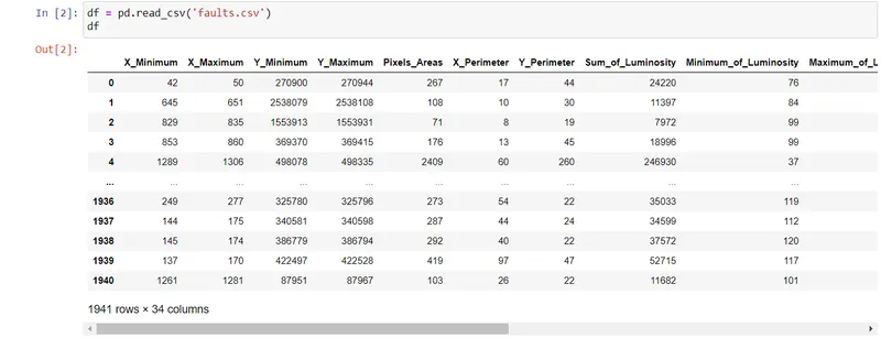
Let's see the description of the data.
df.describe()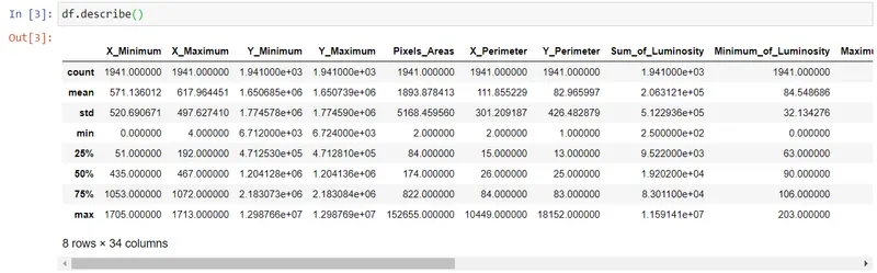
Now let's check what are the different attributes and defects present in the data and their datatypes.
df.info()<class 'pandas.core.frame.DataFrame'>
RangeIndex: 1941 entries, 0 to 1940
Data columns (total 34 columns):
# Column Non-Null Count Dtype
--- ------ -------------- -----
0 X_Minimum 1941 non-null int64
1 X_Maximum 1941 non-null int64
2 Y_Minimum 1941 non-null int64
3 Y_Maximum 1941 non-null int64
4 Pixels_Areas 1941 non-null int64
5 X_Perimeter 1941 non-null int64
6 Y_Perimeter 1941 non-null int64
7 Sum_of_Luminosity 1941 non-null int64
8 Minimum_of_Luminosity 1941 non-null int64
9 Maximum_of_Luminosity 1941 non-null int64
10 Length_of_Conveyer 1941 non-null int64
11 TypeOfSteel_A300 1941 non-null int64
12 TypeOfSteel_A400 1941 non-null int64
13 Steel_Plate_Thickness 1941 non-null int64
14 Edges_Index 1941 non-null float64
15 Empty_Index 1941 non-null float64
16 Square_Index 1941 non-null float64
17 Outside_X_Index 1941 non-null float64
18 Edges_X_Index 1941 non-null float64
19 Edges_Y_Index 1941 non-null float64
20 Outside_Global_Index 1941 non-null float64
21 LogOfAreas 1941 non-null float64
22 Log_X_Index 1941 non-null float64
23 Log_Y_Index 1941 non-null float64
24 Orientation_Index 1941 non-null float64
25 Luminosity_Index 1941 non-null float64
26 SigmoidOfAreas 1941 non-null float64
27 Pastry 1941 non-null int64
28 Z_Scratch 1941 non-null int64
29 K_Scatch 1941 non-null int64
30 Stains 1941 non-null int64
31 Dirtiness 1941 non-null int64
32 Bumps 1941 non-null int64
33 Other_Faults 1941 non-null int64
dtypes: float64(13), int64(21)
memory usage: 515.7 KBLet's check if there are any missing values consist in the data.
df.isna().sum()X_Minimum 0
X_Maximum 0
Y_Minimum 0
Y_Maximum 0
Pixels_Areas 0
X_Perimeter 0
Y_Perimeter 0
Sum_of_Luminosity 0
Minimum_of_Luminosity 0
Maximum_of_Luminosity 0
Length_of_Conveyer 0
TypeOfSteel_A300 0
TypeOfSteel_A400 0
Steel_Plate_Thickness 0
Edges_Index 0
Empty_Index 0
Square_Index 0
Outside_X_Index 0
Edges_X_Index 0
Edges_Y_Index 0
Outside_Global_Index 0
LogOfAreas 0
Log_X_Index 0
Log_Y_Index 0
Orientation_Index 0
Luminosity_Index 0
SigmoidOfAreas 0
Pastry 0
Z_Scratch 0
K_Scatch 0
Stains 0
Dirtiness 0
Bumps 0
Other_Faults 0
dtype: int64Comments:
- There are 1941 data points and 34 features in the dataset out of which 27 are attributes and 6 are defects.
- All the values in the columns are of int and float type only.
- There are no missing values present in the data.
2. Data Visualisation:
We will first divide the data into two part in the pandas dataframe.
Faults = df[['Pastry', 'Z_Scratch', 'K_Scatch', 'Stains', 'Dirtiness', 'Bumps', 'Other_Faults']]
Attributes = df.drop(columns = Faults)
Now we are going to visualise the data to see how it visually looks like.
We will first make pie chart of all Faults dataframe so that we will get to know which type of faults are mostly present and which faults are least present in the dataframe.
plt.subplots(figsize = ([12,12]))
plt.pie(x=Faults.value_counts().sort_values(),autopct = '%.2f%%',labels = Faults.columns)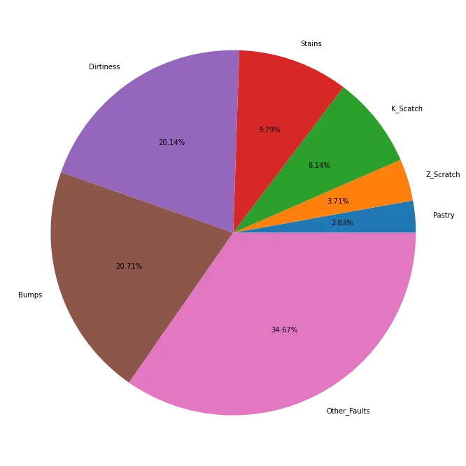
-Pastry fault is the least occuring defect in the steel plates contributing only 2.83% whereas Other_Faults contribute the maximum amount of defects in the steel plates with 34.67%.
We will now plot the histogram plots of all the attributes columns and analyse how the data points are distributes for each attribute.
df.hist(figsize = ([50,50]))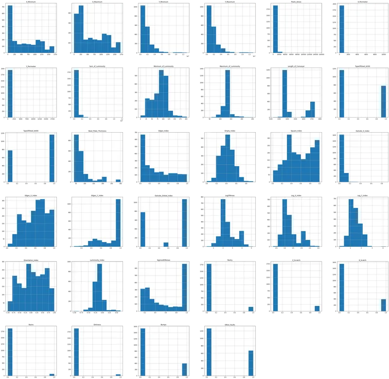
- From the visual inspection of the histogram plots it is observe that maximum number of defects occur when X dimension ranges from 0 to 250 and Y dimension ranges from 0 to 0.3e7.
- The steel plate of type A400 has more number of defects than the steel plates of type A300.
Now we plot a heatmap of all the features so that we can observe the relations between the features in the dataset.
plt.subplots(figsize = ([15,15]))
sns.heatmap(Attributes.corr(),cmap = 'YlGnBu')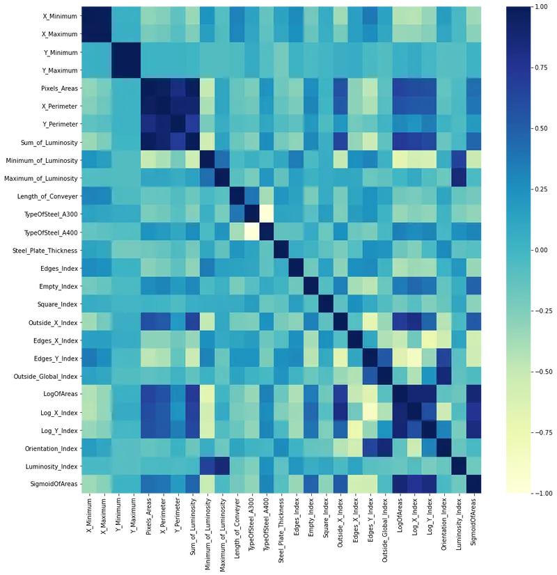
The darkest blue colour indicates the strong correlation between the features.
On inspecting the heatmap we can observe the following correlations between the features:
- Sum of Luminosity and Pixels Areas.
- Log of Areas and Sigmoid of Areas.
- Orientation Index and Outside Global Index.
- Edges Y Index and Outside Global Index.
- Maximum of Luminosity and Luminosity Index.
Comments:
- 34.7% of the defects in the steel plates are known to us so it is categorised as Other_Faults.This fault contributes the maximum number of faults in the dataset.
- The most number of defects are occuring in A400 type Steel plate.So there must be something wrong with this type of steel.
- A strong correlation between some features are observed which must be further analysed.
3. Analysing the correlations between the features:
We will now analyse the correlations between the features which we have listed out above using heat map.
We will use regression plot to analyse whether the features have a actual linear correlations between the features.
sns.regplot(x = df['Sum_of_Luminosity'],y = df['Pixels_Areas'])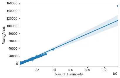
sns.regplot(x = df['LogOfAreas'],y = df['SigmoidOfAreas'])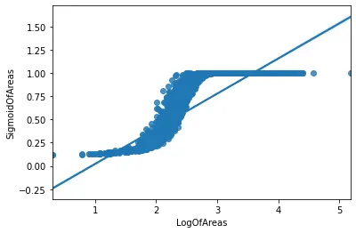
sns.regplot(x = df['Orientation_Index'],y = df['Outside_Global_Index'])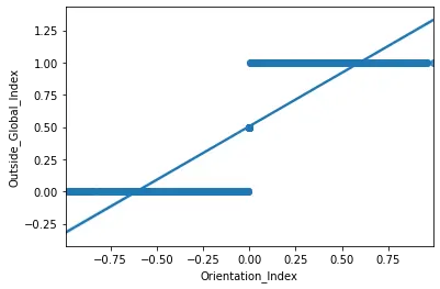
sns.regplot(x = df['Edges_Y_Index'],y = df['Outside_Global_Index'])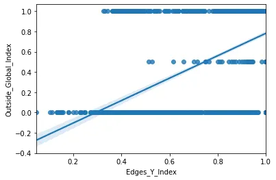
sns.regplot(x = df['Luminosity_Index'],y = df['Maximum_of_Luminosity'])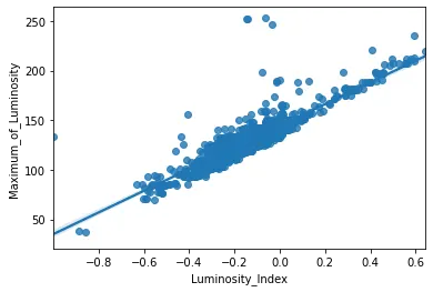
Comments:
- Out of 5 correlations that we have plotted only 3 shows the actual linear correlations between the features. These are:
- Sum of Luminosity and Pixels Areas.
- Log of Areas and Sigmoid of Areas.
- Maximum of Luminosity and Luminosity Index.
4. Analysing Feature Skewness:
Feature skewness tells the amount of skewness in a particular column. Generally it is advised to have normally distributed data so that the algorithm will perform computationally well.
We will now check each and every column which and visualise the most skewed columns.
feature_skewness = pd.DataFrame(Attributes.skew())
feature_skewness.sort_values(ascending = False,by = 0)
0
Y_Perimeter 39.293158
X_Perimeter 21.539451
Pixels_Areas 14.083822
Sum_of_Luminosity 7.730720
Outside_X_Index 5.181830
Y_Minimum 2.811213
Y_Maximum 2.811169
Steel_Plate_Thickness 2.206935
Maximum_of_Luminosity 1.287035
Log_X_Index 1.001014
Length_of_Conveyer 0.851422
LogOfAreas 0.748284
Edges_Index 0.685771
Luminosity_Index 0.679339
X_Maximum 0.524210
X_Minimum 0.500897
Log_Y_Index 0.445101
TypeOfSteel_A300 0.407249
Empty_Index 0.293468
SigmoidOfAreas 0.125789
Square_Index -0.056306
Minimum_of_Luminosity -0.107098
Orientation_Index -0.153446
Edges_X_Index -0.235096
Outside_Global_Index -0.306422
TypeOfSteel_A400 -0.407249
Edges_Y_Index -0.928582By looking at the above data we can say that the Y_perimeter is the most positively skewed column and Edges _Y_Index is the most negatively skewed column.
Now let's visualise them.
sns.distplot(df['Y_Perimeter'])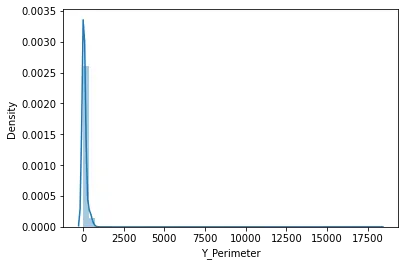
sns.distplot(df['X_Perimeter'])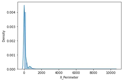
sns.distplot(df['Edges_Y_Index'])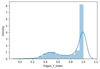
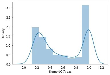
sns.distplot(df['SigmoidOfAreas'])
Comments:
- Y Perimeter and X_Perimeter is the most skewed feature in the positive direction.
- Edges_Y_Index is the most skewed feature in the negative direction.
- Sigmoid Of Areas is the most normalised feature in the dataset.
- Most of the features in the dataset are close to the normal distribution.
5. Analysing Outliers:
An outlier is an observation that lies an abnormal distance from other values in a random sample from a population. In a sense, this definition leaves it up to the analyst (or a consensus process) to decide what will be considered abnormal. Before abnormal observations can be singled out, it is necessary to characterize normal observations.
An outlier acts a noise in the data which is not good for the machine learning algorithms to predict the model.
Boxplot is the best representation for detecting the outliers.
To create the box plot we will first scaled the data as we have large number of data points which will not give a clear picture of the plot.
from sklearn.preprocessing import StandardScaler
scaler = StandardScaler()
Attributes_scaled = pd.DataFrame(scaler.fit_transform(Attributes),columns = Attributes.columns)
Attributes_scaled.boxplot(return_type = 'axes',figsize = (20,20),vert = False)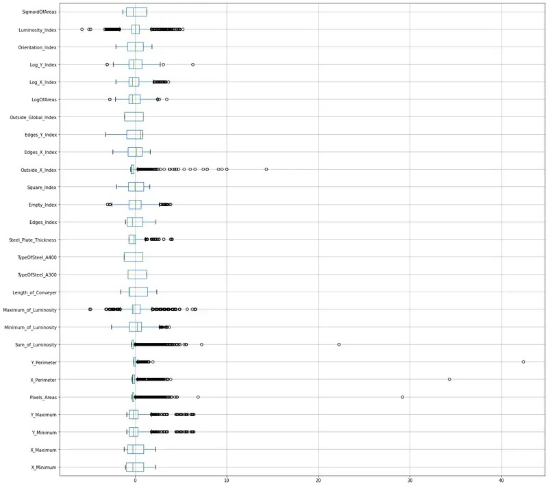
Now we have a clear image of the outliers.
Comments:
- There are many outliers in this dataset which is expected as this is a fault dataset of the steel plates. We cannot remove them right now as the provider of the dataset does not provide the description for the outliers. It can only remove with the help of an expert advice.
6. Summary and Conclusion:
- There are 1941 data points,27 attributes and 6 type of defects in the data.
- There are no missing values found in the data.
- Some unknown faults,Bumps and Dirtiness are the most common type of defects seen in the data.
- The steel plates of type A400 has more number of defects than A300.
- Some correlations can be found between the attributes.
- Y_Perimeter and Edges_Y_Index is the most skewed attributes in the data in positive and negative direction respectively.
- Sigmoid of Areas is the most normally distributed attribute in this data.
- There are many outliers in the data in different attributes which we cannot remove right now due to insufficient knowledge given in the description of this data.It can only be removed if we get any expert knowledge.
Performing SVM:
First of all need to add a new column to the dataset called 'Target' in which we will merge all the faults into one column as SVM algorithm can only be performed with one target column.
Target = []
for i in range(Faults.shape[0]):
    if df['Pastry'].values[i] == 1:
        Target.append('Pastry')
    elif df['Z_Scratch'].values[i] == 1:
        Target.append('X_Scratch')
    elif df['K_Scatch'].values[i] == 1:
        Target.append('K_Scatch')
    elif df['Stains'].values[i] == 1:
        Target.append('Stains')
    elif df['Dirtiness'].values[i] == 1:
        Target.append('Dirtiness')
    elif df['Bumps'].values[i] == 1:
        Target.append('Bumps')
    else:
        Target.append('Other_Faults')

Target = pd.DataFrame(Target)
df['Target'] = Target
Now we are ready to perform EVM on our dataset.
The data set is splitting into two dataset namely training and test dataset in 70%:30% ratio.
We will use Attributes_scaled dataset for further procedure as the orignal data takes forever to run the model.
from sklearn.model_selection import train_test_split

X_train,X_test,y_train,y_test = train_test_split(Attributes_scaled,Target,test_size = 0.3,random_state = 4)
Applying the SVM model to our training dataset.
from sklearn import svm
model = svm.SVC(C = 1,kernel = 'linear',gamma = 'auto')
fit_model = model.fit(X_train,y_train)
Now we will measure the accuracy of our model and try some predictions of the test data.
score = fit_model.score(X_test,y_test)
score0.7341337907375644y_predict = fit_model.predict(X_test)
y_predictarray(['Other_Faults', 'K_Scatch', 'Bumps', 'Other_Faults',
'Other_Faults', 'Bumps', 'K_Scatch', 'Bumps', 'K_Scatch',
'K_Scatch', 'Bumps', 'Other_Faults', 'Other_Faults',
'Other_Faults', 'X_Scratch', 'Other_Faults', 'K_Scatch',
'X_Scratch', 'Other_Faults', 'Other_Faults', 'Other_Faults',
'Bumps', 'Bumps', 'K_Scatch', 'X_Scratch', 'Bumps', 'X_Scratch',
'Other_Faults', 'Other_Faults', 'X_Scratch', 'K_Scatch',
'Other_Faults', 'K_Scatch', 'X_Scratch', 'Bumps', 'Pastry',
'Stains', 'Other_Faults', 'K_Scatch', 'Pastry', 'Other_Faults',
'Pastry', 'K_Scatch', 'Stains', 'Bumps', 'Other_Faults', 'Bumps',
'Other_Faults', 'X_Scratch', 'Other_Faults', 'Other_Faults',
'K_Scatch', 'K_Scatch', 'Bumps', 'Bumps', 'Bumps', 'Other_Faults',
'Other_Faults', 'Dirtiness', 'K_Scatch', 'Other_Faults', 'Bumps',
'Bumps', 'Bumps', 'Other_Faults', 'Bumps', 'K_Scatch', 'K_Scatch',
'Other_Faults', 'Other_Faults', 'Bumps', 'X_Scratch', 'Stains',
'Other_Faults', 'X_Scratch', 'Other_Faults', 'K_Scatch',
'X_Scratch', 'Bumps', 'Bumps', 'K_Scatch', 'Bumps', 'Other_Faults',
'Bumps', 'Bumps', 'Stains', 'Bumps', 'Other_Faults',
'Other_Faults', 'K_Scatch', 'K_Scatch', 'Other_Faults', 'K_Scatch',
'Other_Faults', 'Bumps', 'Bumps', 'Bumps', 'Other_Faults',
'Other_Faults', 'Bumps', 'Bumps', 'Dirtiness', 'Bumps',
'Other_Faults', 'Pastry', 'Bumps', 'Bumps', 'K_Scatch', 'Bumps',
'Other_Faults', 'Other_Faults', 'Bumps', 'Other_Faults',
'Other_Faults', 'Pastry', 'K_Scatch', 'Bumps', 'Other_Faults',
'Other_Faults', 'Other_Faults', 'K_Scatch', 'Other_Faults',
'Other_Faults', 'Other_Faults', 'K_Scatch', 'Pastry', 'Bumps',
'Pastry', 'Bumps', 'Other_Faults', 'K_Scatch', 'Bumps', 'Bumps',
'Bumps', 'Pastry', 'Other_Faults', 'Other_Faults', 'Bumps',
'K_Scatch', 'Other_Faults', 'K_Scatch', 'Other_Faults', 'K_Scatch',
'K_Scatch', 'Bumps', 'Stains', 'Bumps', 'Other_Faults',
'X_Scratch', 'Bumps', 'Other_Faults', 'Other_Faults',
'Other_Faults', 'Other_Faults', 'Other_Faults', 'Other_Faults',
'Bumps', 'Bumps', 'Other_Faults', 'Pastry', 'Other_Faults',
'K_Scatch', 'Other_Faults', 'K_Scatch', 'Bumps', 'Other_Faults',
'Other_Faults', 'Stains', 'Other_Faults', 'X_Scratch', 'X_Scratch',
'Bumps', 'K_Scatch', 'Bumps', 'K_Scatch', 'Other_Faults', 'Bumps',
'Other_Faults', 'Other_Faults', 'Other_Faults', 'Pastry', 'Bumps',
'Bumps', 'Bumps', 'Other_Faults', 'Bumps', 'K_Scatch', 'K_Scatch',
'X_Scratch', 'Other_Faults', 'Bumps', 'Bumps', 'K_Scatch',
'Other_Faults', 'K_Scatch', 'Other_Faults', 'K_Scatch',
'Other_Faults', 'X_Scratch', 'Other_Faults', 'K_Scatch',
'Other_Faults', 'Bumps', 'Other_Faults', 'Other_Faults',
'K_Scatch', 'Other_Faults', 'Other_Faults', 'K_Scatch', 'Bumps',
'K_Scatch', 'Other_Faults', 'X_Scratch', 'K_Scatch', 'Pastry',
'Other_Faults', 'Other_Faults', 'Pastry', 'Bumps', 'K_Scatch',
'Dirtiness', 'Bumps', 'K_Scatch', 'Other_Faults', 'Bumps',
'K_Scatch', 'K_Scatch', 'Stains', 'Bumps', 'K_Scatch', 'X_Scratch',
'Bumps', 'Other_Faults', 'Other_Faults', 'Pastry', 'Other_Faults',
'Bumps', 'Bumps', 'K_Scatch', 'K_Scatch', 'Other_Faults', 'Stains',
'K_Scatch', 'Other_Faults', 'Other_Faults', 'Bumps',
'Other_Faults', 'Bumps', 'Other_Faults', 'K_Scatch',
'Other_Faults', 'Bumps', 'Other_Faults', 'Bumps', 'Bumps',
'K_Scatch', 'Other_Faults', 'X_Scratch', 'Bumps', 'Other_Faults',
'X_Scratch', 'Other_Faults', 'Bumps', 'Other_Faults', 'X_Scratch',
'Bumps', 'K_Scatch', 'Other_Faults', 'Other_Faults', 'K_Scatch',
'Bumps', 'X_Scratch', 'Other_Faults', 'K_Scatch', 'X_Scratch',
'X_Scratch', 'K_Scatch', 'K_Scatch', 'X_Scratch', 'Bumps',
'Other_Faults', 'K_Scatch', 'Other_Faults', 'Other_Faults',
'Pastry', 'Other_Faults', 'K_Scatch', 'Bumps', 'K_Scatch',
'Other_Faults', 'Dirtiness', 'Other_Faults', 'K_Scatch', 'Bumps',
'K_Scatch', 'Pastry', 'X_Scratch', 'Other_Faults', 'Other_Faults',
'Pastry', 'Other_Faults', 'K_Scatch', 'K_Scatch', 'Bumps', 'Bumps',
'Other_Faults', 'Bumps', 'Other_Faults', 'K_Scatch', 'K_Scatch',
'K_Scatch', 'Bumps', 'Other_Faults', 'X_Scratch', 'Other_Faults',
'Bumps', 'X_Scratch', 'X_Scratch', 'K_Scatch', 'Dirtiness',
'Pastry', 'X_Scratch', 'K_Scatch', 'Pastry', 'Other_Faults',
'Dirtiness', 'K_Scatch', 'Bumps', 'X_Scratch', 'K_Scatch',
'Other_Faults', 'Other_Faults', 'X_Scratch', 'Stains', 'K_Scatch',
'Bumps', 'X_Scratch', 'Bumps', 'Other_Faults', 'K_Scatch',
'X_Scratch', 'K_Scatch', 'K_Scatch', 'K_Scatch', 'Other_Faults',
'K_Scatch', 'Other_Faults', 'Bumps', 'K_Scatch', 'K_Scatch',
'Other_Faults', 'Other_Faults', 'Bumps', 'Bumps', 'Other_Faults',
'Other_Faults', 'K_Scatch', 'X_Scratch', 'Other_Faults', 'Bumps',
'Other_Faults', 'Other_Faults', 'Other_Faults', 'K_Scatch',
'Other_Faults', 'Other_Faults', 'Other_Faults', 'X_Scratch',
'Other_Faults', 'Other_Faults', 'Other_Faults', 'Bumps',
'X_Scratch', 'Dirtiness', 'Other_Faults', 'Bumps', 'Bumps',
'Bumps', 'Bumps', 'Bumps', 'Bumps', 'Bumps', 'Other_Faults',
'Other_Faults', 'Other_Faults', 'X_Scratch', 'Bumps',
'Other_Faults', 'K_Scatch', 'X_Scratch', 'K_Scatch', 'Bumps',
'Bumps', 'Other_Faults', 'Other_Faults', 'Other_Faults',
'Other_Faults', 'Other_Faults', 'Bumps', 'Other_Faults', 'Bumps',
'K_Scatch', 'Bumps', 'Other_Faults', 'Other_Faults', 'Bumps',
'Other_Faults', 'Other_Faults', 'X_Scratch', 'Other_Faults',
'K_Scatch', 'K_Scatch', 'Other_Faults', 'Other_Faults', 'K_Scatch',
'K_Scatch', 'Bumps', 'Other_Faults', 'K_Scatch', 'X_Scratch',
'Other_Faults', 'Bumps', 'Other_Faults', 'K_Scatch', 'Bumps',
'Dirtiness', 'Other_Faults', 'K_Scatch', 'X_Scratch',
'Other_Faults', 'Other_Faults', 'X_Scratch', 'Bumps',
'Other_Faults', 'K_Scatch', 'Pastry', 'K_Scatch', 'Bumps',
'Other_Faults', 'Bumps', 'Pastry', 'Pastry', 'Bumps',
'Other_Faults', 'Bumps', 'Other_Faults', 'X_Scratch', 'K_Scatch',
'K_Scatch', 'Other_Faults', 'Other_Faults', 'X_Scratch',
'Other_Faults', 'Other_Faults', 'Other_Faults', 'Pastry', 'Bumps',
'Other_Faults', 'Bumps', 'Other_Faults', 'Other_Faults',
'K_Scatch', 'K_Scatch', 'K_Scatch', 'Other_Faults', 'X_Scratch',
'Other_Faults', 'K_Scatch', 'Stains', 'K_Scatch', 'Bumps',
'K_Scatch', 'Pastry', 'Other_Faults', 'Other_Faults', 'K_Scatch',
'K_Scatch', 'Stains', 'X_Scratch', 'Pastry', 'K_Scatch', 'Stains',
'Bumps', 'Bumps', 'Other_Faults', 'K_Scatch', 'Bumps',
'Other_Faults', 'Bumps', 'Other_Faults', 'Bumps', 'K_Scatch',
'Pastry', 'K_Scatch', 'K_Scatch', 'Bumps', 'K_Scatch',
'Other_Faults', 'Other_Faults', 'K_Scatch', 'Pastry',
'Other_Faults', 'Other_Faults', 'Pastry', 'Pastry', 'X_Scratch',
'Pastry', 'Other_Faults', 'Other_Faults', 'K_Scatch', 'K_Scatch',
'K_Scatch', 'Other_Faults', 'Other_Faults', 'Other_Faults',
'X_Scratch', 'K_Scatch', 'Pastry', 'Other_Faults', 'K_Scatch',
'Bumps', 'Other_Faults', 'K_Scatch', 'Bumps', 'Other_Faults',
'Other_Faults', 'Other_Faults', 'Other_Faults', 'Other_Faults',
'Bumps', 'X_Scratch', 'K_Scatch', 'X_Scratch', 'K_Scatch', 'Bumps',
'Bumps', 'Pastry', 'Other_Faults', 'Other_Faults', 'K_Scatch',
'Other_Faults', 'Dirtiness', 'Other_Faults', 'Bumps', 'K_Scatch',
'Other_Faults', 'Other_Faults', 'Pastry', 'X_Scratch',
'Other_Faults', 'Bumps', 'X_Scratch', 'Other_Faults', 'K_Scatch',
'K_Scatch', 'Other_Faults', 'Other_Faults', 'K_Scatch', 'Stains',
'K_Scatch', 'Other_Faults', 'Pastry', 'K_Scatch', 'Bumps', 'Bumps',
'K_Scatch', 'Other_Faults', 'Other_Faults', 'Bumps', 'Dirtiness',
'X_Scratch', 'Bumps', 'K_Scatch', 'Bumps', 'Pastry',
'Other_Faults', 'K_Scatch', 'K_Scatch', 'X_Scratch',
'Other_Faults', 'Bumps', 'Other_Faults', 'Bumps'], dtype='<U12')Let's create a confusion matrix to visualise the properly.
from sklearn import metrics
cm = metrics.confusion_matrix(y_test,y_predict)
cm = pd.DataFrame(cm,columns = Faults.columns)
cm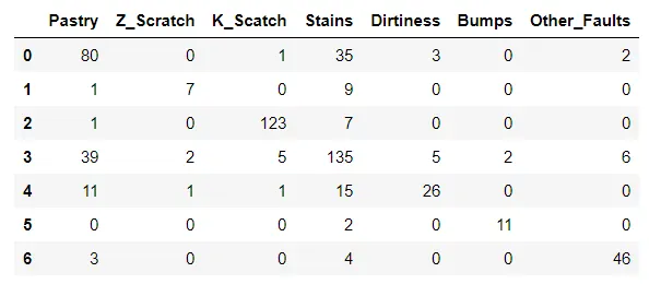
plt.figure(figsize = (20,20))
sns.heatmap(cm,annot = True,xticklabels = cm,yticklabels = cm)
plt.xlabel('Y Actual')
plt.ylabel('Y Predict')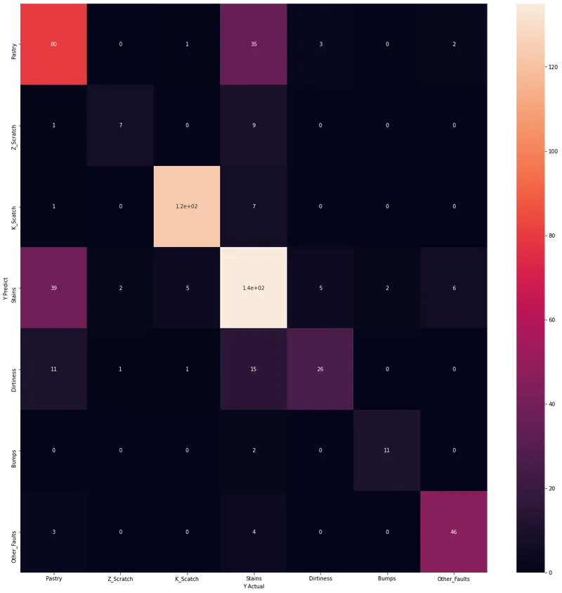
Summary and Conclusion:
- The dataset was first scaled and divided into training and test dataset.
- The accuracy of the model was found out to be 73.4%.
- The comparison of actual data and predicted data is carried out with the help of a confusion matrix.
- Confusion matrix shows that most errors occurs in the prediction of 'Stains' defects and least errors occurs in the prediction of 'Other_faults'.