Flow over a Cylinder.

Objective:

• To simulate the flow over a cylinder and explain the phenomenon of Karman vortex street.
• To simulate the flow with the steady and unsteady case and calculate the Strouhal Number for Re= 100.
• To calculate the coefficient of drag and lift over a cylinder by setting the Reynolds number to 10,100,1000,10000 & 100000 and running it with the steady solver.
• To discuss the effect of Reynolds number on the coefficient of drag.

Karman Vortex Street:

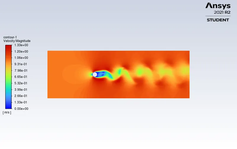
In fluid dynamics, a Kármán vortex street (or a von Kármán vortex street) is a repeating pattern of swirling vortices, caused by a process known as vortex shedding, which is responsible for the unsteady separation of flow of a fluid around blunt bodies.

It is named after the engineer and fluid dynamicist Theodore von Kármán, and is responsible for such phenomena as the "singing" of suspended telephone or power lines and the vibration of a car antenna at certain speeds.

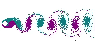
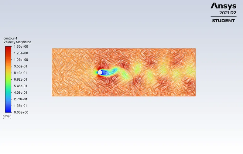
Vortex shedding is an oscillating flow that takes place when a fluid such as air or water flows past a bluff (as opposed to streamlined) body at certain velocities, depending on the size and shape of the body. In this flow, vortices are created at the back of the body and detach periodically from either side of the body forming a Von Kármán vortex street. The fluid flow past the object creates alternating low-pressure vortices on the downstream side of the object. The object will tend to move toward the low-pressure zone.

If the bluff structure is not mounted rigidly and the frequency of vortex shedding matches the resonance frequency of the structure, then the structure can begin to resonate, vibrating with harmonic oscillations driven by the energy of the flow. This vibration is the cause for overhead power line wires humming in the wind, and for the fluttering of automobile whip radio antennas at some speeds. Tall chimneys constructed of thin-walled steel tubes can be sufficiently flexible that, in air flow with a speed in the critical range, vortex shedding can drive the chimney into violent oscillations that can damage or destroy the chimney.

Vortex shedding was one of the causes proposed for the failure of the original Tacoma Narrows Bridge (Galloping Gertie) in 1940, but was rejected because the frequency of the vortex shedding did not match that of the bridge. The bridge actually failed by aeroelastic flutter.

A thrill ride, "VertiGo" at Cedar Point in Sandusky, Ohio suffered vortex shedding during the winter of 2001, causing one of the three towers to collapse. The ride was closed for the winter at the time. In northeastern Iran, the Hashemi-Nejad natural gas refinery's flare stacks suffered vortex shedding seven times from 1975 to 2003. Some simulation and analyses were done, which revealed that the main cause was the interaction of the pilot flame and flare stack. The problem was solved by removing the pilot.

The frequency at which vortex shedding takes place for an infinite cylinder is related to the Strouhal number by the following equation:

Where is the dimensionless Strouhal number, is the vortex shedding frequency (s^-1), is the diameter of the cylinder (m), and is the flow velocity (m s^-1).

The Strouhal number depends on the Reynolds number , but a value of 0.22 is commonly used. Over four orders of magnitude in Reynolds number, from 100 to 100000, the Strouhal number varies only between 0.18 and 0.22.

To validate the Strouhal number analytically we have the formula:

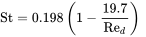
This formula will generally hold true for the range 250 < Re_d < 200000.

Simulating the Karman Vortex street in Ansys Fluent:

• We will be going to simulate the flow over a cylinder for the steady and unsteady cases. For both the cases we have to calculate the Strouhal number using simulation and validating the results with the analytical formula for the Strouhal Number only for Re = 100.
• Then after the simulation for steady and unsteady flow for Re = 100, we will simulate the flow over a cylinder for the Reynolds number Re = 10,100,1000,10000 & 100000 using the steady state solver.
• We will plot the results for drag coefficient, lift coefficient & vertex average.
• For the simulation we will be performing the following procedure:

1. Geometry Creation.
2. Meshing.
3. Problem Setup.
4. Solving.
5. Post-Processing.

• Finally we will discuss the effect of Reynold's number on the coefficient of drag.

1. Geometry Creation:

The required geometry for the simulation is going to be created in a Ansys module called Spaceclaim.

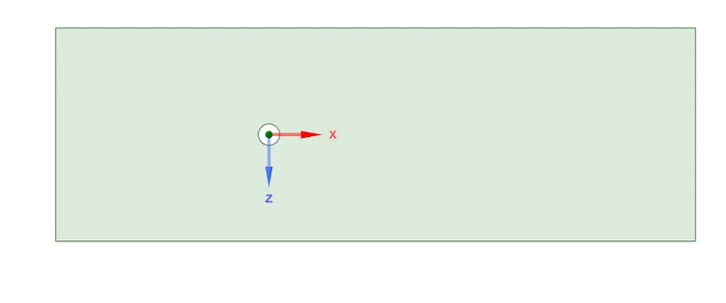
The diameter of the cylinder is 2m and there will be a rectangle around the cylinder. The geometry is shown below:

2. Meshing:

In the next step we will be doing the meshing the geomertry created in the previous step.

We have to open the mesh module of the fluent module and we can see that the geometry has been imported there automatically.

• In the first step we have to name the edges, so we will select the edges and presses N and start to name the edges. The front boundary is named as inlet, the rear boundary is named as outlet, the cylinder edge is named as walls and the upward/downward boundary are named as symmetry.
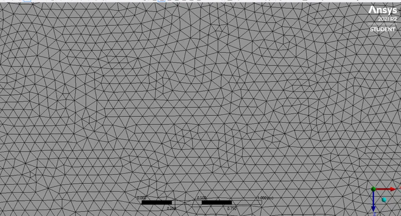
• After the above step we will set the mesh shape to be triangulated by right clicking the mesh option and then go for the method. We are choosing the element size to be 0.08m.

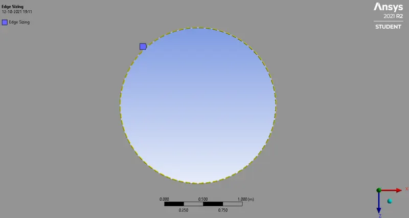
• Now after the meshing we will do the sizing of the cylinder edge to make it a perfect circle.
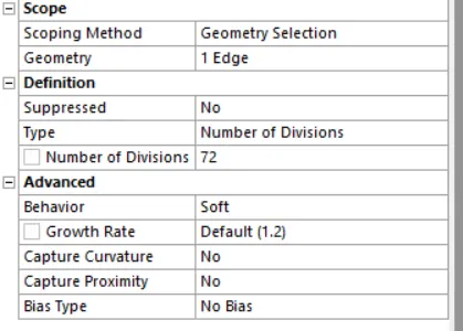
• We will right click on the mesh and then select Sizing. We will select the type of the sizing as Number of Divisions and enter 72 number of divisions.

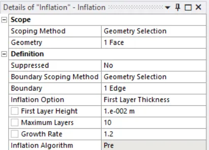
• In the next step of meshing we will do the inflation around the cylinder edge. Inflation layer helps to create a body fitted mesh i.e. it creates a number of layers around the cylider body to provide some thickness to it.
• To do that we first right click on the mesh branch and then select the Inflation option. We will enter 0.001m as the first layer height and 10 be the maximum number of layers.

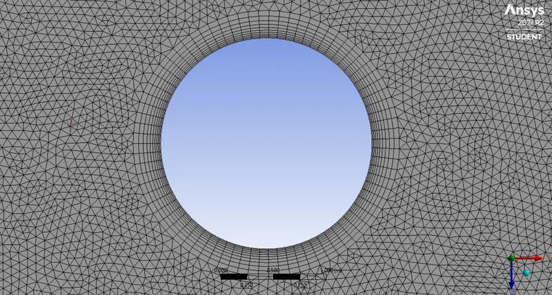
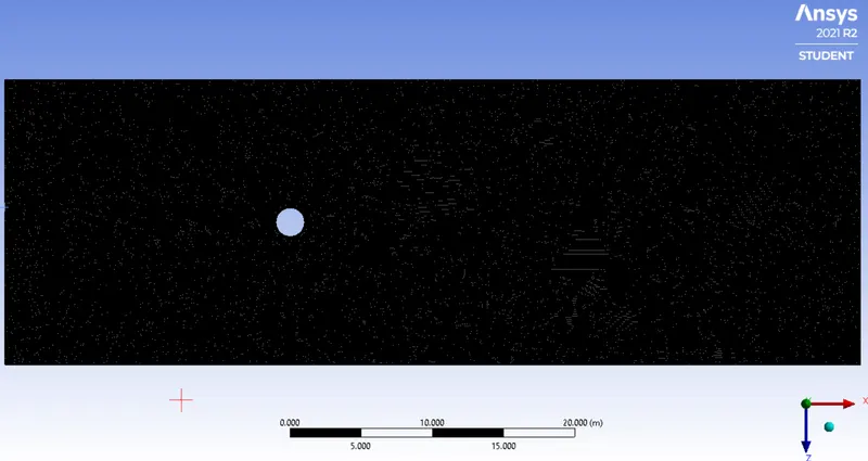
The final mesh is shown below:

3. Problem Setup:

This is the next step after meshing the geometry to setup the model ready for simulations. In this process we have to esblish the physics of the problem like setting up the initial condition,boundary condition, setting the materials, etc.

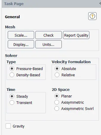
We first set the general settings as shown below:

Now we will move to the physics tab where we will be going to set up the following things:

• Setting up the Viscous model.
• Creating a new material.
• Setting up the Cell zones and Boundary Conditions.

Setting up the Viscous model:

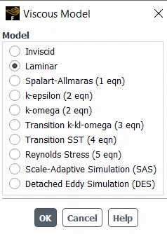
We will be selecting the Viscous model as Laminar as shown below:

Creating a new material:

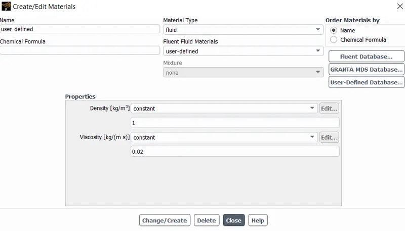
We will create a user defined material whose Density is 1 kg/m3 and a dynamic viscosity according to the fomula:

`R_e = (rhoUL)/mu`

where,

`rho = 1 kg//m^3`

U = 1 m/s,

L = 2 m.

The value of `mu` will decide the Reynold's number we require. For e.g,

If we have the requirement of Re = 100 then we will enter the value of `mu = 0.02` so that we get the desired Reynold's number.

Setting up the cell zones and boundary conditions:

Cell zone: In the cell zone we will be having the option to change the fluid material which we have created.

Boundary Conditions:

In this section we will be defining the boundary conditions at inlet,cylinder walls and outlet.

Inlet: Velocity = 1m/s.

Outlet: Pressure = 0 gauge.

Cylinder Walls: Wall = No Slip.

After defining the boundary conditions we will go to the Solution tab to run the Simulations.

Before running the simulation we will need to have some plots for the drag, lift and vertex average. To do that we first create a monitor point at 4D downstream the cylinder. In the result tab we will go to the surface section and create a point from there, where X = 8 m and Y = 0.

After creating the monitor point we will create the reports for drag, lift and vertex average at the monitor point.

At last we will create an animation file to visualize the vortex formation. For that we will got to the solution tab click on create -> solution animation from the Activities section. We will capture the frame after every 10 iterations for the velocity contour.

To create the contours we will go to the results tab and click on Contours -> New from the graphics section, then we will select all the boundaries in the contour menu and click OK. And that contour file will be used in the animation of the flow.

4. Solving:

• In this procedure we will first initialise the program at t = 0.
• Now we will enter 3000 iterations for the steady state solver and for the unsteady solver we will set the number of time steps be 300 with the step size of 0.25.
• Now we are ready to run the Simulations.

5. Post Processing:

This is the final step of the simulation where we have to analyse the solutions after running all the cases.

The cases we are going to run are divided into Part 1 and Part 2. In Part 1 we are run for Steady and Unsteady state of the flow with Reynold's number 100 and also calculating the Strouhal number.

In Part 2 we will run the Steady state flow for the Reynold's number 10,1000,10000, & 100000.

Part 1: Simulating the flow with the steady and unsteady case and calculate the Strouhal Number for Re= 100.

(i). Steady State Flow for Re = 100.

Residual Plots:

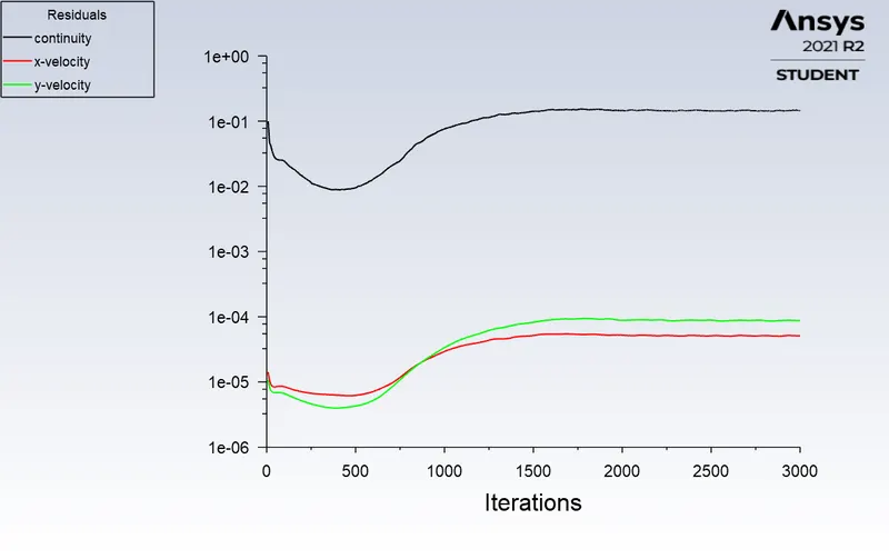
It has been observed from the above plot that the residuals are converged after 1000 iterations.

Vertex Average plot:

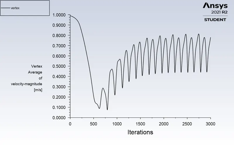
We can observe from the above plot that the vertex average plot is converged after 1500 iterations and become steady state.

Drag plot:

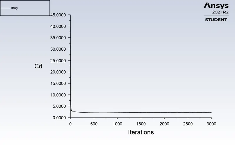
So from the above plot it has been concluded that the drag coefficient does not change and it remains constant throughout the simulation. In other words, the plot is converged.

Lift plot:

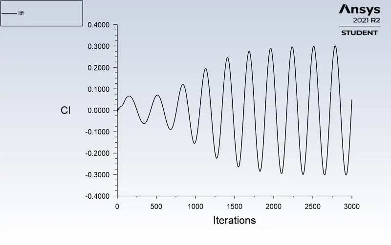
It has been observed that the plot achieved the steady state after 1500 iterations, so it is concluded that the plot is converged.

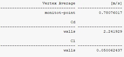
Report results:

Velocity Contour:

(ii). Unsteady state flow at Re = 100.

Residual Plots:

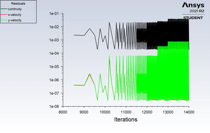
It has been observed from the above plot that the residuals are converged after 13000 iterations.

Vertex Average plot:

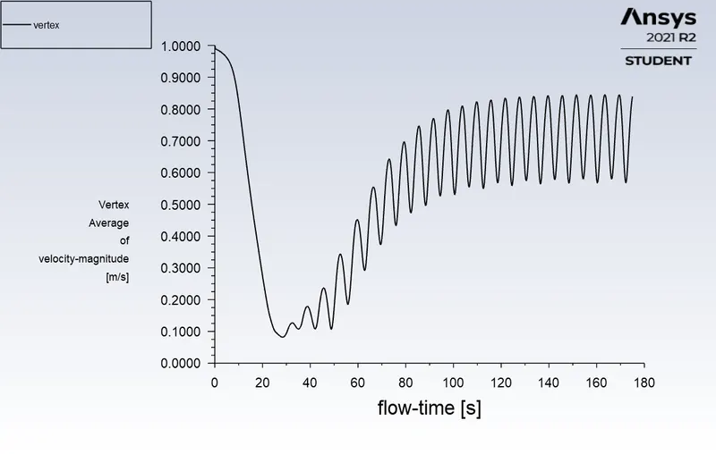
We can observe from the above plot that the vertex average plot is converged after 120 sec of flow time and become steady state.

Drag plot:

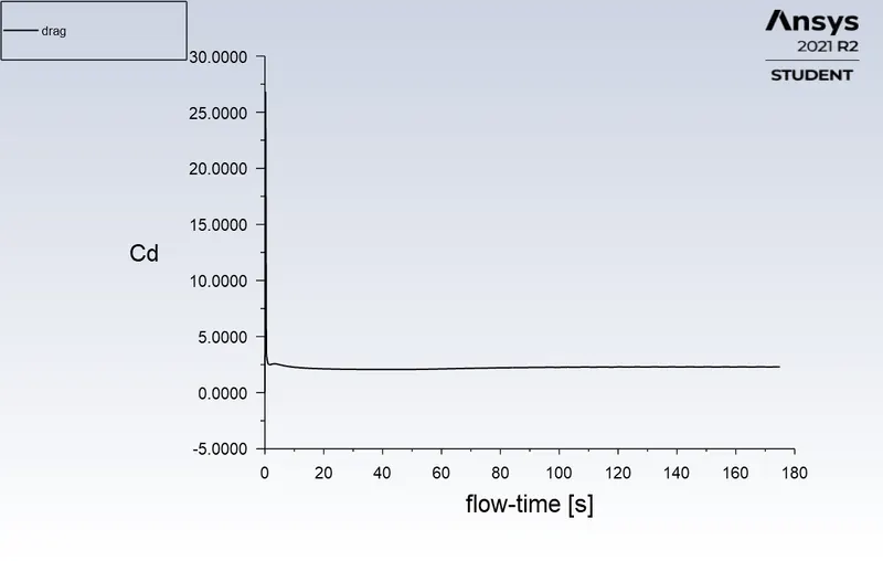
So from the above plot it has been concluded that the drag coefficient does not change and it remains constant throughout the simulation. In other words, the plot is converged.

Lift plot:

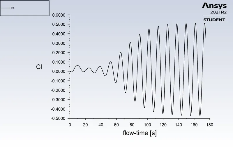
It has been observed that the plot achieved the steady state after 120 sec of flow time, so it is concluded that the plot is converged.

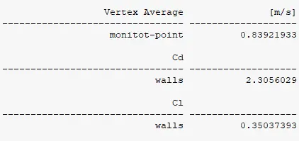
Report results:

Velocity Contour:

Calculating the Strouhal number:

We know that the Strouhal number is expressed by the formula:

Where is the dimensionless Strouhal number, is the vortex shedding frequency (s^-1), is the diameter of the cylinder (m), and is the flow velocity (m s^-1).

It is already givem that V = 1 m/s and D = 2 m.

The vortex shedding frequency is calculated by the lift plot by the formula, f = no.of cycles/time period,

We can observe from the Lift plot there are 4 no. of complete cycles from 120 s to 170 s . So, the time period is 50 s and the vortex shedding frequency is calculated as f = 4/50 = 0.08.

Now from the Simulation thee Strouhal number is calculated as:

`St = (0.08xx2)/1 = 0.16`

To validate this result we will calculate the Strouhakl number by the formula:

Where Re = 100.

`St = 0.198(1-(19.7)/100) = 0.159`

`=>` So the value of Strouhal number is validated by the analytical method and it is observed that both the values are approximately equal.

Part 2: Calculating the coefficient of drag and lift over a cylinder by setting the Reynolds number to 10,1000,10000 & 100000 using Steady state solver.

Case 1: Reynolds Number = 10

Residual Plots:

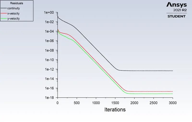
It has been observed from the above plot that the residuals are converged after 1750 iterations.

Vertex Average plot:

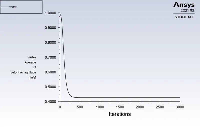
We can observe from the above plot that the vertex average plot is converged after 500 iterations and become steady state.

Drag plot:

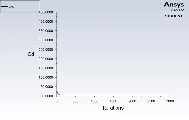
So from the above plot it has been concluded that the drag coefficient does not change and it remains constant throughout the simulation. In other words, the plot is converged.

Lift plot:

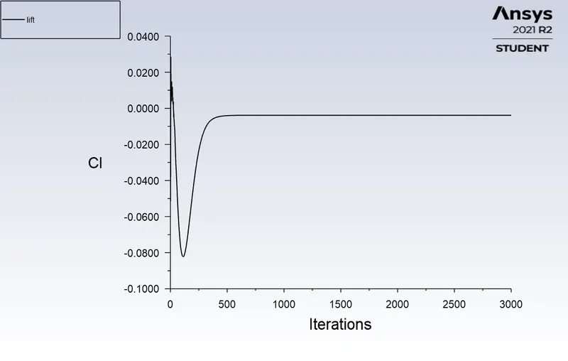
It has been observed that the plot achieved the steady state after 500 iterations, so it is concluded that the plot is converged.

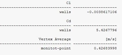
Report results:

Velocity Contour:

Case 2: Reynold's number = 1000.

Residual Plots:

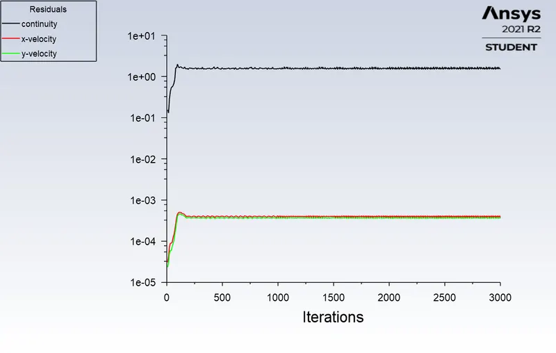
It has been observed from the above plot that the residuals are converged after 250 iterations.

Vertex Average plot:

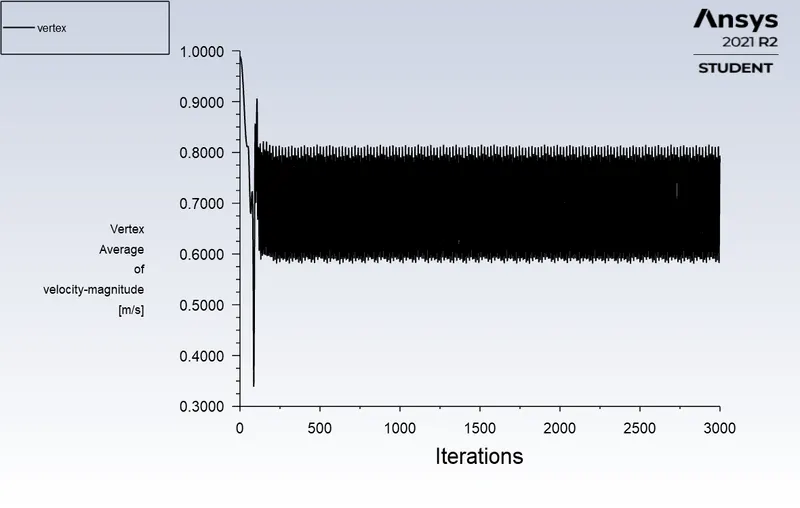
We can observe from the above plot that the vertex average plot is converged after 250 iterations and become steady state.

Drag plot:

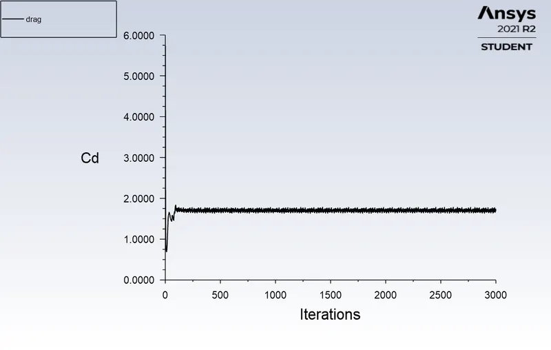
So from the above plot it has been concluded that the drag coefficient become steady after 250 iterations. In other words, the plot is converged.

Lift plot:

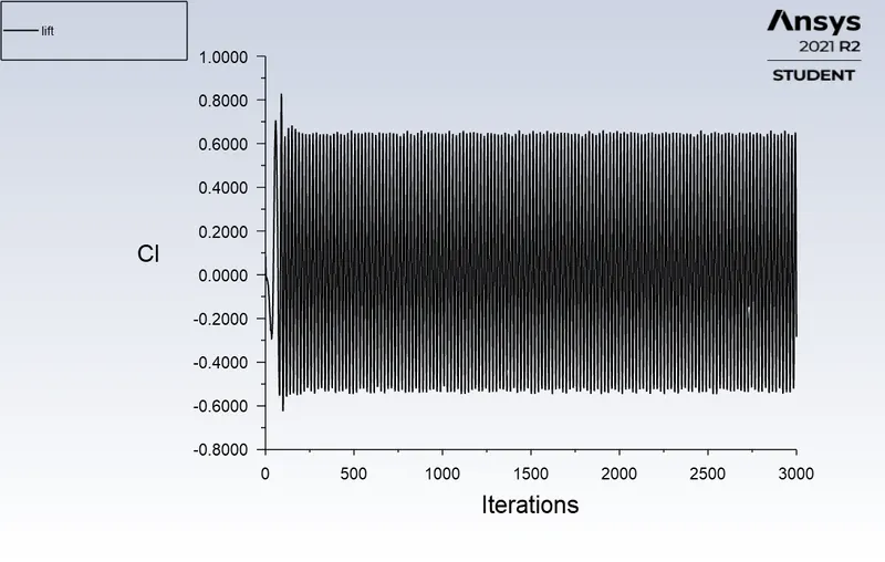
It has been observed that the plot achieved the steady state after 100 iterations, so it is concluded that the plot is converged.

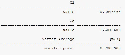
Report results:

Velocity Contour:

Case 3: Reynold's Number = 10000.

Residual Plots:

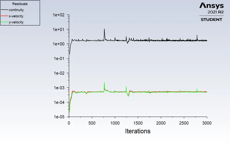
It has been observed from the above plot that the residuals are converged after 1500 iterations.

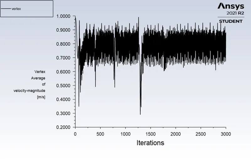
Vertex Average plot:

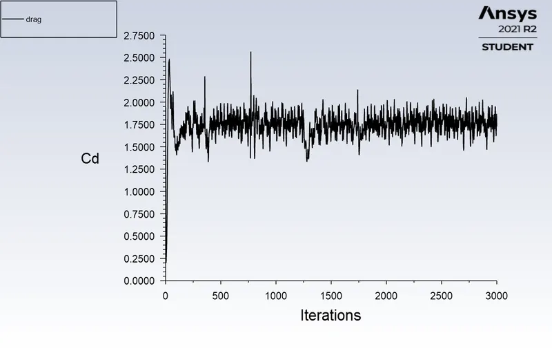
Drag plot:

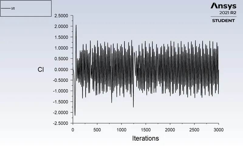
Lift plot:

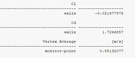
Report results:

Velocity Contour:

Case 4: Reynold's Number = 100000

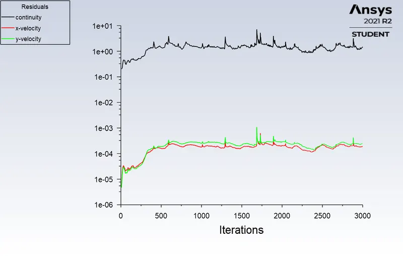
Residual Plots:

Vertex Average plot:

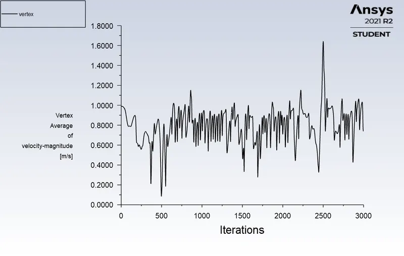
We can observe from the above plot that the vertex average plot is converged after 1500 iterations and become steady state.

Drag plot:

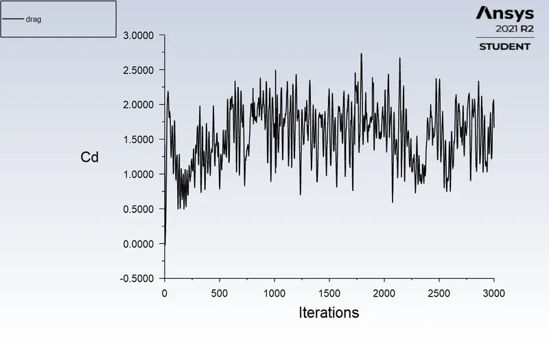
Lift plot:

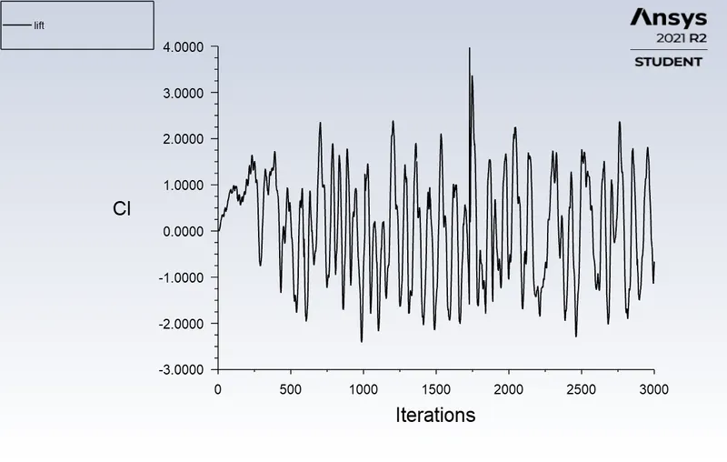
Report results:

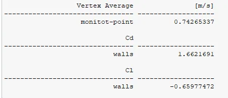
Velocity Contour:

Observations:

Reynold's Number	Drag Coefficient	Lift Coefficient	Vertex Average in m/s
10	5.42	-0.003	0.42
100	2.24	0.05	0.78
1000	1.68	-0.28	0.78
10000	1.73	-0.02	0.88
100000	1.66	-0.65	0.74

• At Re = 10, we can observe that the flow is seperated but remains steady. It shows how the votices occurs at low velocity. The vortices formed downstream of the flow are stable.
• At Re = 100, the flow is steadily seperated at the begining and then started to form vortices. It shows how the fluid flows over the cylinder at some increased velocity.
• At Re = 1000, the velocity is increased even more and the drag began to lower down due to this the vortices are formed and reached the steady state quite early.
• At Re = 10000 & 100000, the velocity is extremely high due to this the vortices formed immidiately after the cylinder in a very rigorous manner. The drag becomes even smaller and the loss of velocity downstream is lower.

Effect of Reynold's Number on Drag Coefficient:

After running all the cases and looking at the observation table it has been concluded that the drag coefficient is inversely proportional to the Reynold's Number. As the Reynold's number increases the drag coefficient decreases linearly.