Mixing Tee Simulation using Ansys Fluent
Objective:
- To set up steady-state simulations to compare the mixing effectiveness when hot inlet temperature is 360C & the Cold inlet is at 190C.
- To use K-omega and K-epsilon models and compare them to obtain the best suitable model for the given case.
- To perform the mesh independent study for anyone case.
- To discuss the effect of length and momentum ratio on results.
Mixing Tees:
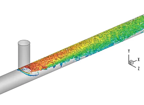
Mixing tees—in which two fluid streams with different physical and/or chemical properties mix—are widely used in the petrochemical industry. When there is a large temperature difference between two streams, large metal temperature fluctuations can occur in the region where the two streams meet if proper design steps are not taken. The temperature fluctuations in the metal can lead to thermal fatigue of the pressure boundary piping. If through-wall cracking occurs, the fluid may leak, possibly causing a fire and damage. Therefore, it is imperative to ensure that the piping system can withstand the temperature fluctuations. Options can include improving the mixing of the two streams to reduce the temperature fluctuations through redesign of the piping system such that the momentum ratio of the two fluid streams is favorable to rapid mixing, or installing devices that protect the pressure boundary piping (e.g., injection quills or thermal sleeves in the region where the temperature fluctuations are higher than a thermal fatigue threshold). This region includes the T-junction and a length of differing main pipe diameters downstream from the T-junction.
K-epsilon turbulent model:
The K-epsilon model is one of the most common turbulence models, although it just doesn't perform well in cases of large adverse pressure gradients. It is a two equation model, that means, it includes two extra transport equations to represent the turbulent properties of the flow. This allows a two equation model to account for history effects like convection and diffusion of turbulent energy.
The first transported variable is turbulent kinetic energy, . The second transported variable in this case is the turbulent dissipation, . It is the variable that determines the scale of the turbulence, whereas the first variable, , determines the energy in the turbulence.
There are two major formulations of K-epsilon models. That of Launder and Sharma is typically called the "Standard" K-epsilon Model. The original impetus for the K-epsilon model was to improve the mixing-length model, as well as to find an alternative to algebraically prescribing turbulent length scales in moderate to high complexity flows.
The K-epsilon model has been shown to be useful for free-shear layer flows with relatively small pressure gradients. Similarly, for wall-bounded and internal flows, the model gives good results only in cases where mean pressure gradients are small; accuracy has been shown experimentally to be reduced for flows containing large adverse pressure gradients. One might infer then, that the K-epsilon model would be an inappropriate choice for problems such as inlets and compressors.
K-omega turbulent model:
The k-omega (k−ω) turbulence model is one of the most commonly used models to capture the effect of turbulent flow conditions. It belongs to the Reynolds-averaged Navier-Stokes (RANS) family of turbulence models where all the effects of turbulence are modeled.
It is a two-equation model. That means in addition to the conservation equations, it solves two transport equations (PDEs), which account for the history effects like convection and diffusion of turbulent energy. The two transported variables are turbulent kinetic energy (k), which determines the energy in turbulence, and specific turbulent dissipation rate (ω), which determines the rate of dissipation per unit turbulent kinetic energy. ω is also referred to as the scale of turbulence.
The standard k−ω model is a low Re model, i.e., it can be used for flows with low Reynolds number where the boundary layer is relatively thick and the viscous sublayer can be resolved.
Thus, the standard k−ω model is best used for near-wall treatment. Other advantages include a superior performance for complex boundary layer flows under adverse pressure gradients and separations (e.g., external aerodynamics and turbomachinery). On the contrary, this model has also shown to predict excessive and early separations.
There exist different variations of the k-omega model such as standard k-omega (discussed above), baseline k-omega, k-omega SST, etc., each with certain modifications to perform better under certain conditions of the fluid flow.
SST stands for shear stress transport. The SST formulation switches to a k−ϵ behavior in the free-stream, which avoids the k−ω problem of being sensitive to the inlet free-stream turbulence properties.
The k−ω SST model provides a better prediction of flow separation than most RANS models and also accounts for its good behavior in adverse pressure gradients. It has the ability to account for the transport of the principal shear stress in adverse pressure gradient boundary layers. It is the most commonly used model in the industry given its high accuracy to expense ratio.
On the negative side, the SST model produces some large turbulence levels in regions with large normal strain, like stagnation regions and regions with strong acceleration. This effect is much less pronounced than with a normal k-epsilon model though.
Case Studies:
There are mainly two cases that we have to perform the simulation one for the shorter length T-pipe and one for the longer length T-pipe. But we also have to run the simulations for different momentum ratios and different turbulent models so in total we have to run 5 cases.
| Cases | Momentum Ratios | Length | Turbulent Model |
| Case 1 | 2 | Short | K-epsilon |
| Case 2 | 2 | Short | K-omega |
| Case 3 | 4 | Short | - |
| Case 4 | 2 | Long | - |
| Case 5 | 4 | Long | - |
We have to put '-' from Case 3 onwards because we first have to decide which turbulence model is more preferable than the other.
Case Set-up:
In the case set-up procedure we will be preparing our geometry ready for the simulation.
1. Geometry import:
We first have to import the gemoetry into the Ansys Spaceclaim.
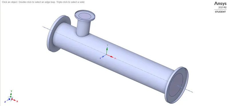
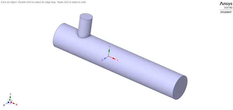
Now we have to extract the geometry suitable for the simulation where the fluid actually flows.
2. Setting -up for Meshing:
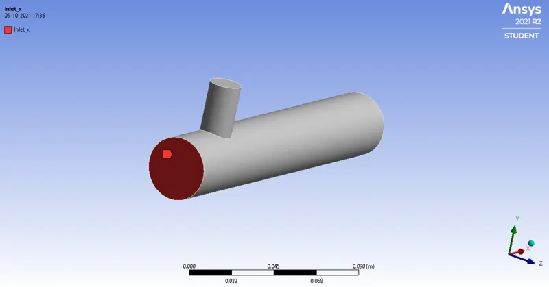
In this step we will be going to name the surfaces of the geometry before meshing.
The name of the surfaces are given as follows:
(i). Inlet_x:
This is the name of the surface where hot air of `36^oC` temperature will enter.
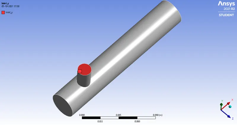
(ii). Inlet_y:
This is the name of the surface where cold air of `19^oC` temperature will enter.
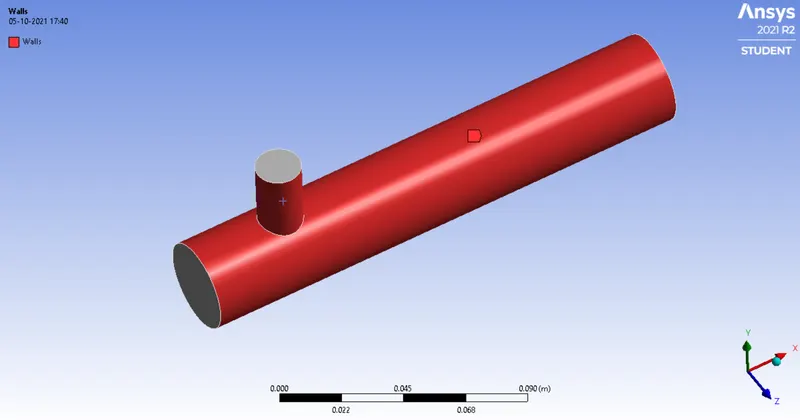
(iii). Wall:
These are the walls of the pipes:
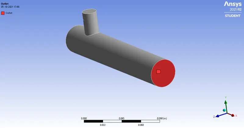
(iv). Outlet:
This is the outlet of the pipe.
Case 1:
Parameters:
| Length | Short |
| Momentum Ratio | 2 |
| Hot air velocity with temperarure | 3m/s ; `36^oC` |
| Cold Air velocity with temperature | 6m/s ; `19^oC` |
| Element Size | 5e-3 |
| Number of Elements | 14250 |
| Turbulence Model | K-epsilon (Realizable) |
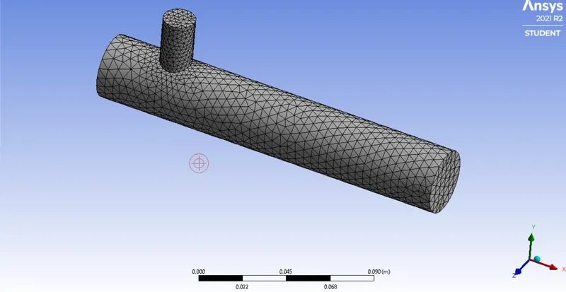
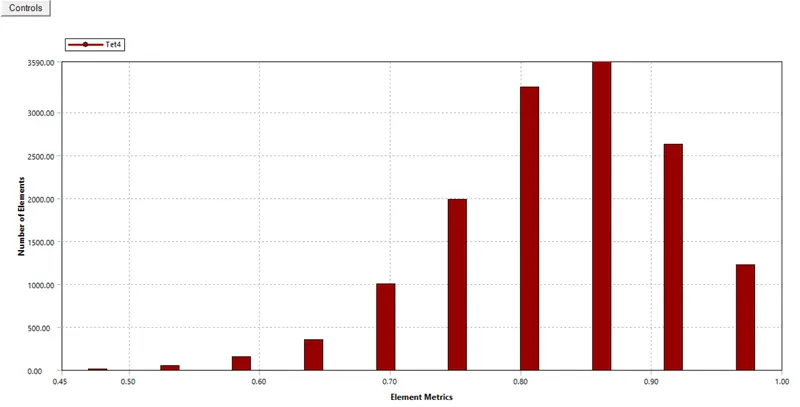
Note: As we are going to choose the element size of 5e-03 in every case, the mesh and the mesh quality plot is going to be the same for every case.
Mesh:
Mesh Quality:
Solutions:
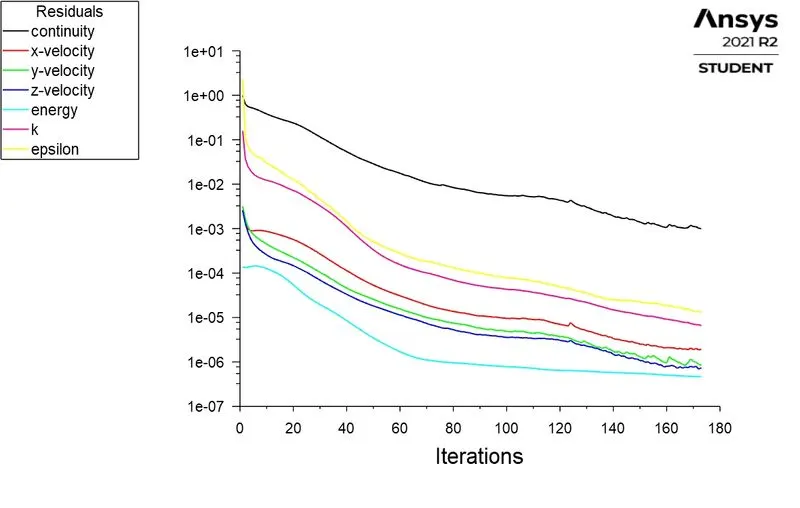
Residuals plot:
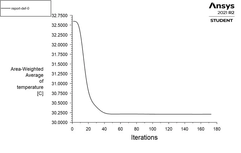
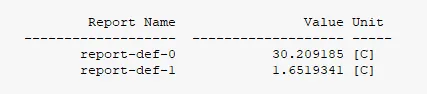
Area-Weighted Average of Temperature:
Standard Deviation of Temperature:
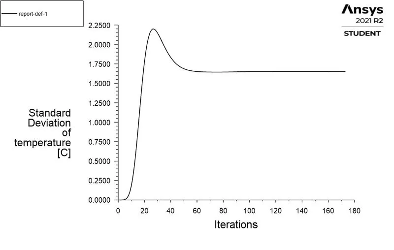
We can observe from the above plots that almost all the plots are converged after 160-180 iterations
Post-processing:
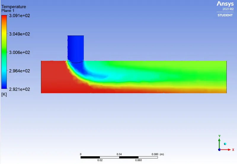
1. Temperature contours:
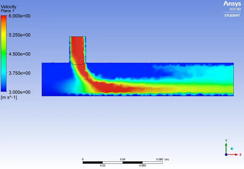
2. Velocity:
Case 2:
Parameters:
| Length | Short |
| Momentum Ratio | 2 |
| Hot air velocity with temperarure | 3m/s ; `36^oC` |
| Cold Air velocity with temperature | 6m/s ; `19^oC` |
| Element Size | 5e-3 |
| Number of Elements | 14250 |
| Turbulence Model | K-omega (SST) |
Solutions:
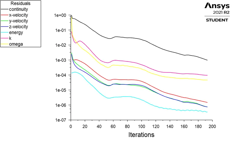
Residual Plot:
Area-Weighted Average of Temperature:
Standard Deviation of Temperature:
Post-processing:
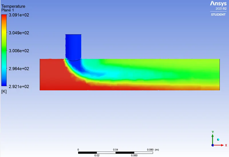
1. Temperature contour:
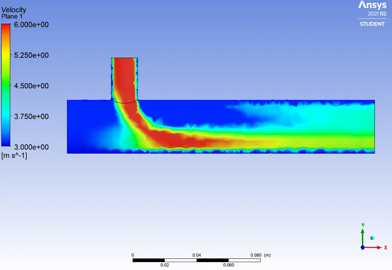
2. Velocity Contour:
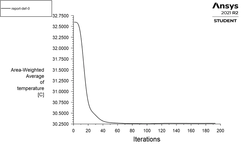
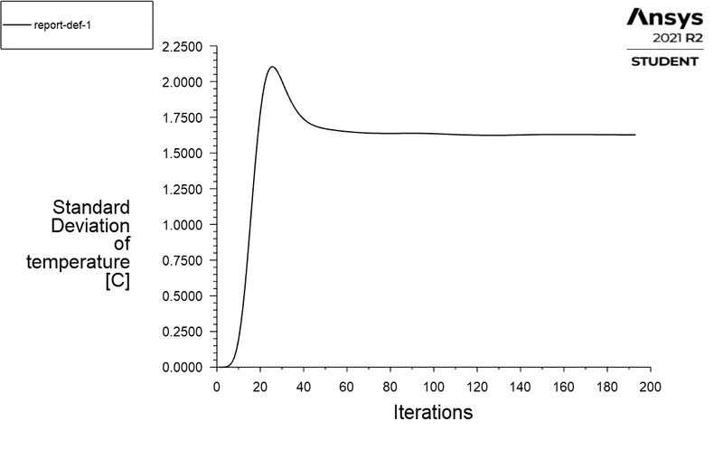
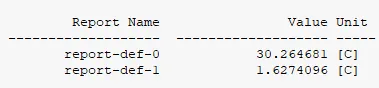
From the above simulation in Case 2 we have observed that the residual plots took nearly 180-200 iterations to converge, area-weighted average of temperature plot took nearly 70-80 interations to converge and standard deviation of temperature took nearly 100-120 iterations to converge.
Analytical Solution of the mixture:
The temperature at the outlet of the tee-pipe is given as,
Given data,
`T_(hot) = 36^oC, and T_(cold)=19^oC`
Momentum ratio is 2,
`V_(hot) = 3m//s, V_(cold) = 6 m//s`
`m_(hot) = rhoA_(hot)V_(hot) = 1.225xx225.9131xx3 = 3313.0959 kg//s`
`m_(cold) = rhoA_(cold)V_(cold) = 1.225xx225.9131xx6 =1660.4612 kg//s`
`T_(mixture) = (3313.0959xx36 +1660.4612xx19)/(3313.0959 + 1660.4612)`
`T_(mixture) = 32.32^oC`
Comparison between case 1 and case 2:
| Cases | Turbulence model | Momentum Ratio | Tee-Length | No. of Elements | Outlet Temperature(Area-weighted) | Standard Deviation of the outlet temperature | No. of Iterations |
| Case 1 | K-epsilon | 2 | Short | 14250 | 30.20 C | 1.65 | 160-180 |
| Case 2 | K-omega | 2 | Short | 14250 | 30.26 C | 1.63 | 180-200 |
Comments:
We can observe from the above comparison that the results obtained by both the turbulence model are almost the same except K-omega took more number of iterations to converge than the K-epsilon turbulence model. In other words, the K-epsilon turbulence model is more efficient than K-omega model in terms of time taken to complete the simulation.
So we are going to choose K-epsilon model for simulation of the rest of the cases left.
From now the complete table of the cases we need to peform is represented as:
| Cases | Momentum Ratios | Length | Turbulent Model |
| Case 1 | 2 | Short | K-epsilon |
| Case 2 | 2 | Short | K-omega |
| Case 3 | 4 | Short | K-epsilon |
| Case 4 | 2 | Long | K-epsilon |
| Case 5 | 4 | Long | K-epsilon |
Case 3:
Parameters:
| Length | Short |
| Momentum Ratio | 4 |
| Hot air velocity with temperarure | 3m/s ; `36^oC` |
| Cold Air velocity with temperature | 12m/s ; `19^oC` |
| Element Size | 5e-3 |
| Number of Elements | 14250 |
| Turbulence Model | K-epsilon (Realizable) |
Residual Plot:
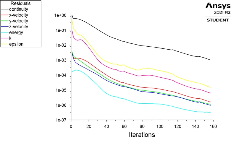
- Total no. of iterations taken = 157.
Area Weighted Average of Temperature:
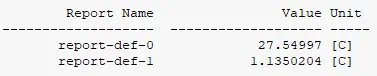
Standard Deviation of Temperature:
Analytical Solution of the mixture:
The temperature at the outlet of the tee-pipe is given as,
Given data,
`T_(hot) = 36^oC, and T_(cold)=19^oC`
Momentum ratio is 4,
`V_(hot) = 3m//s, V_(cold) = 12 m//s`
`m_(hot) = rhoA_(hot)V_(hot) = 1.225xx225.9131xx3 = 3313.0959 kg//s`
`m_(cold) = rhoA_(cold)V_(cold) = 1.225xx225.9131xx6 =3320.9225 kg//s`
`T_(mixture) = (3313.0959xx36 +3320.9225xx19)/(3313.0959 +3320.9225)`
`T_(mixture) = 27.48^oC`
Post-processing:
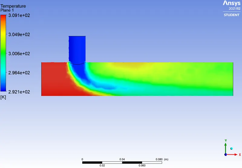
1. Temperature Contour:
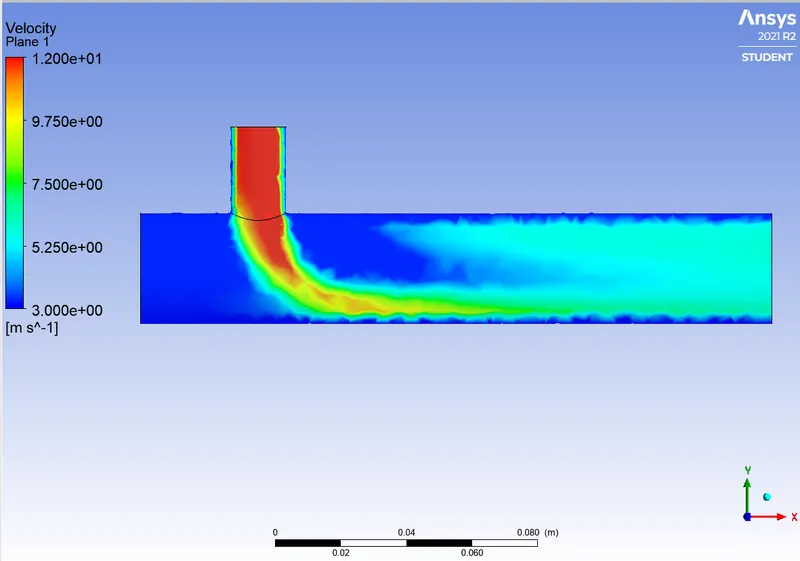
2. Velocity Contour:
Case 4:
Parameters:
| Length | Long |
| Momentum Ratio | 2 |
| Hot air velocity with temperarure | 3m/s ; `36^oC` |
| Cold Air velocity with temperature | 6m/s ; `19^oC` |
| Element Size | 5e-3 |
| Number of Elements | 14250 |
| Turbulence Model | K-epsilon (Realizable) |
Residual Plot:
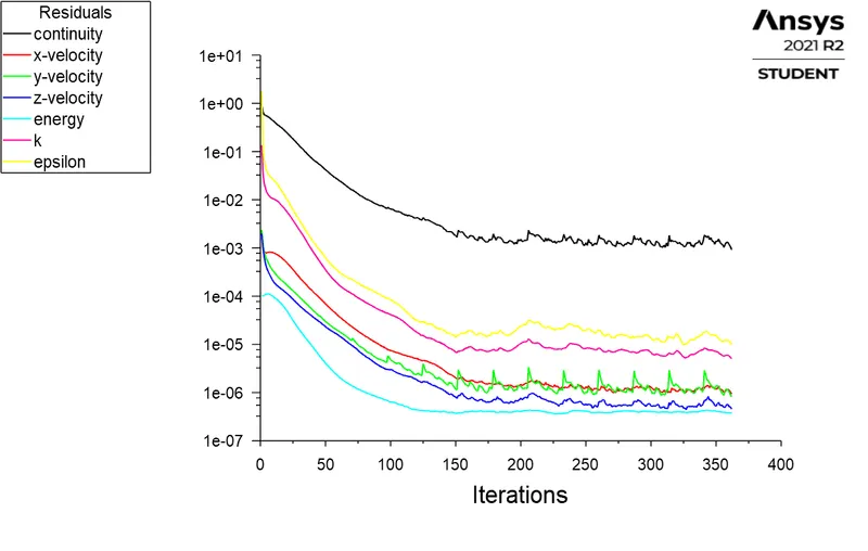
- Total no. of iterations taken = 157.
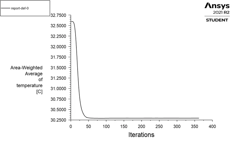
Area Weighted Average of Temperature:
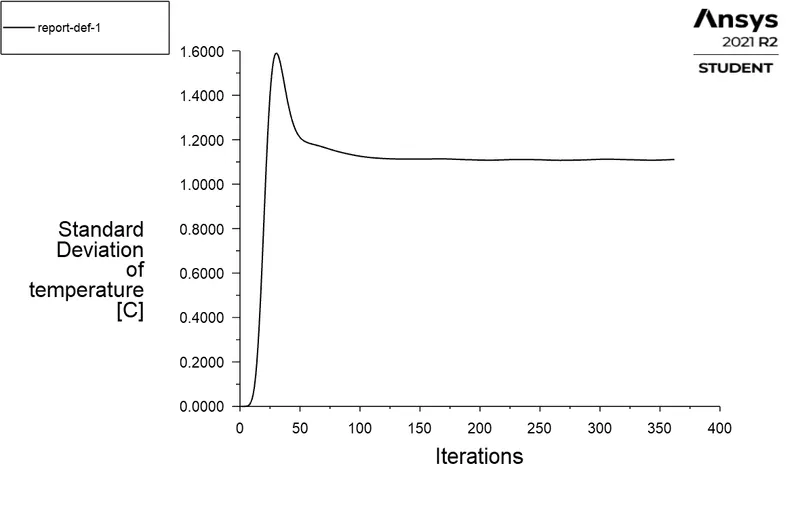
Standard Deviation of Temperature:
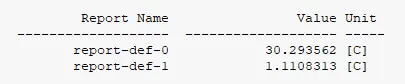
- Total number of iterations taken = 362
Post-Processing:
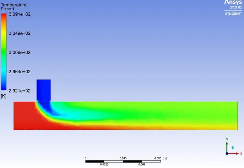
1. Temperature Contour:
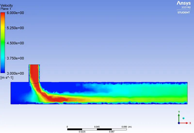
2. Velocity Contour:
Case 5:
Parameters:
| Length | Long |
| Momentum Ratio | 4 |
| Hot air velocity with temperarure | 3m/s ; `36^oC` |
| Cold Air velocity with temperature | 12m/s ; `19^oC` |
| Element Size | 5e-3 |
| Number of Elements | 14250 |
| Turbulence Model | K-epsilon (Realizable) |
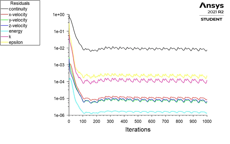
Residual Plot:
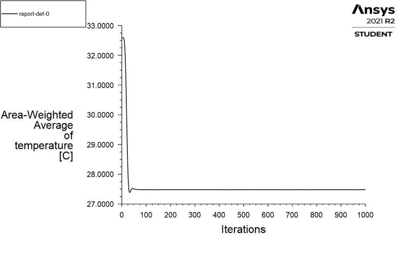
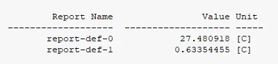
Area-Weighted Average of temperature:
Standard deviation of temperature:
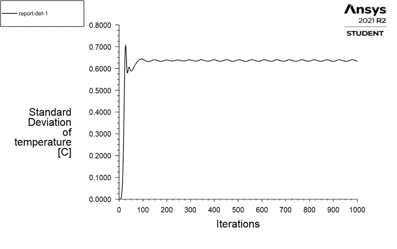
The Simulation ran for 1000 iterations but still doesn't get the converged solution.
Post-processing:
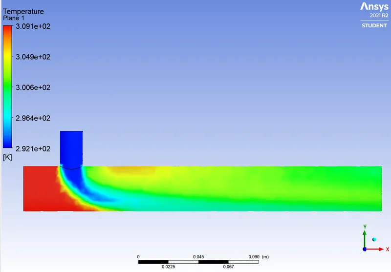
1. Temperature contour:
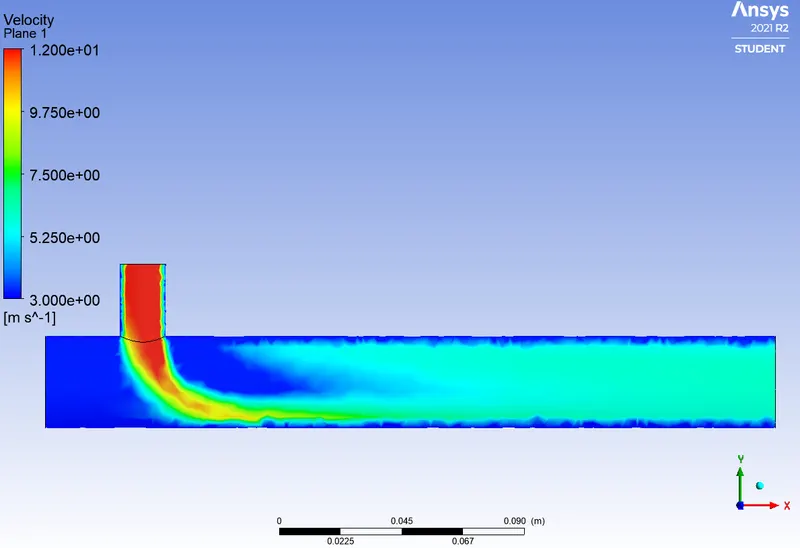
2. Velocity Contour:
Observations:
| Cases | Turbulence model | Momentum Ratio | Tee-Length | No. of Elements | Outlet Temperature(Area-weighted) | Standard Deviation of the outlet temperature | No. of Iterations |
| Case 1 | K-epsilon | 2 | Short | 14250 | 30.20 C | 1.65 C | 160-180 |
| Case 2 | K-omega | 2 | Short | 14250 | 30.26 C | 1.63 C | 180-200 |
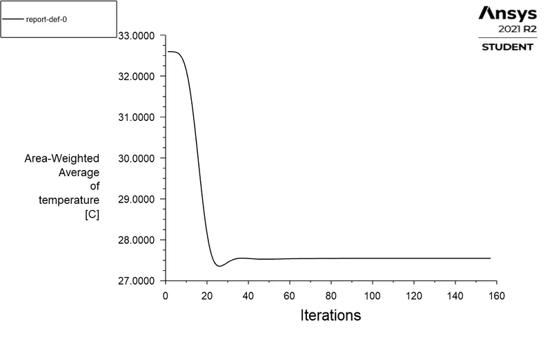
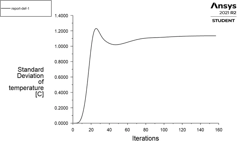
| Case 3 | K-epsilon | 4 | Short | 14250 | 27.55 C | 1.13 C | 157 |
| Case 4 | K-epsilon | 2 | Long | 14250 | 30.29 C | 1.11 C | 362 |
| Case 5 | K-epsilon | 4 | Long | 14250 | 27.48 C | 0.633 C | 1000 (Solution not converged) |
- K-epsilon turbulence model is more time efficient than the K-omega turbulence model.
- In case 3 where the momentum ratio is 4 the solution is converged at 157 no. of iterations whereas in case 5 where the tee-length is long, the solution obtained is exactly equal to the analytical solution and has the lowest standard deviation of temperature. But the solution does not achieve steady state even at 1000 no. of iterations.
- In case 4, the tee-length is long and the solution gets closest to the analytical solution with momentum ratio 2.
- After observing all these facts from the simulation we came to a conclusion that although the no. of iterations taken by the longer tee-length is more than the shorter tee-length but the more accurate results are obtained in case of the longer tee-length instead of shorter tee-length.
Conclusion:
- The simulation of mixing tee is performed in Ansys Fluent.
- All the cases have been set up for the steady state simulations.
- Both the turbulence models K-epsilon and K-omega are compared for better results.
- All the neccessary plots have been attached to support our discussion.
- All the observatios are tabulated and explained in detail.