CHT Analysis on Exhaust port

Objective:

• To give a brief description about Conjugate Heat Transfer (CHT) Analysis.
• To simulate the flow and heat transfer to the solid on an exhaust port.
• To calculate the wall/surface heat transfer coefficient on the internal solid surface & show the velocity & temperature contours in appropriate areas.
• To verify the HTC predictions from the simulation.

Conjugate Heat Transfer (CHT) analysis:

The Conjugate Heat Transfer (CHT) analysis type allows for the simulation of heat transfer between solid and fluid domains by exchanging thermal energy at the interfaces between them. Typical applications of this analysis type exist as, but are not limited to, the simulation of heat exchangers, cooling of electronic equipment, and general-purpose cooling and heating systems.

Conjugate heat transfer is a type of heat transfer analysis between solids and fluid(s). This type of heat transfer includes both convection (between fluids) and conductive (between solids) heat transfer, as well as both forced and natural convection. Common applications and use cases of this thermal simulation type include electronics cooling, heat exchangers, industrial machinery, some AEC cases, and more.

Heat Transfer Coefficient (HTC):

Heat transfer coefficient is a quantitative characteristic of convective heat transfer between a fluid medium (a fluid) and the surface (wall) flowed over by the fluid. This characteristic appears as a proportionality factor a in the Newton-Richmann relation

What is Y+ and why do we need it?

The behaviour of the flow near the wall is a complicated phenomenon and to distinguish the different regions near the wall the concept of wall has been formulated. Thus is a dimensionless quantity, and is distance from the wall measured in terms of viscous lengths.

One of the reasons for the need of is to distinguish different regions near the wall or in the viscous region, however how exactly it helps in turbulence modelling or in general CFD modelling need to be well understood. Let us try to understand this with an example. A fisherman uses fishing net, a grid kind of structure to trap the fishes. If he is trying to catch medium to big sized fishes the grids in the net he uses is somewhat big, but if he is trying to trap even small sized fishes then the grid size of the net should be small enough to capture them. In this case even the large fishes are also captured. Similarly coming back to our case if we intend to resolve the effects near the wall i.e., in the viscous sub layer then the size of the mesh size should be small and dense enough near the wall so that almost all the effects are captured. But in some cases if the wall effects are negligible then there is option of including semi-empirical formulae to bridge between the viscosity affected region and fully turbulent region and in this case the mesh need not to be dense or small near the wall i.e., coarse mesh would work.

Considering the first case i.e., near wall modelling it is well-known that the mesh size should be small enough, however then the question follows is how small ? Thus, here comes the concept of , and based on the value the first cell height can be calculated. The near wall region is meshed using the calculated first cell height value with gradual growth in the mesh so that the effects are captured and avoiding overall heavy mesh count.

Simulation of flow in an exhaust port:

This simulation will be completed in the following steps:

• Geometry Preperation.
• Meshing.
• Problem Set-up.
• Solving.
• Postprocessing.

1. Geometry preperation.

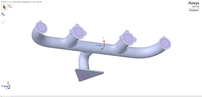
• Firstly, the exhaust port geometry is imported in the Ansys SpaiceClaim and the fluid volume should be extracted.

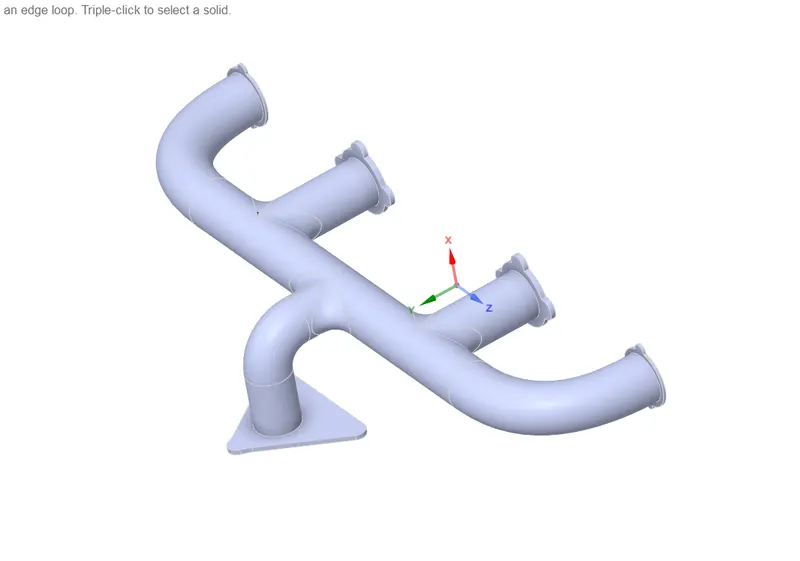
• Now we will extract the fluid volume out of the geometry.

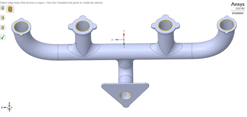
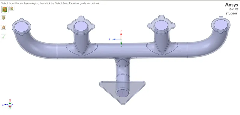
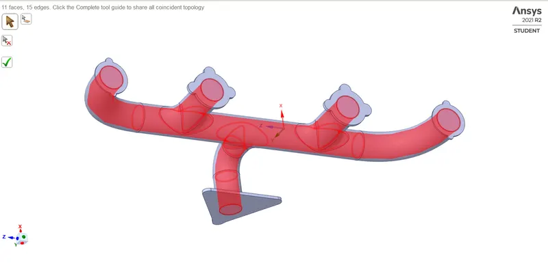
• The fluid volume and the solid volume should share the topology so that the mesh would be evenly generated.

2. Mesh Generation:

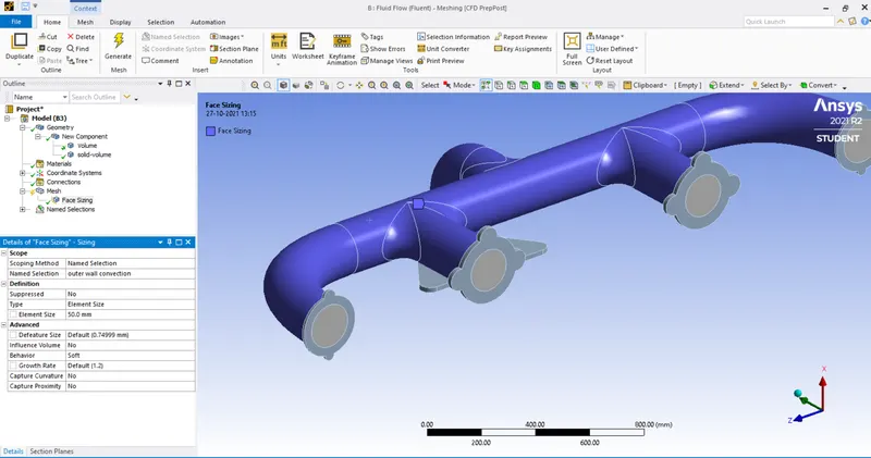
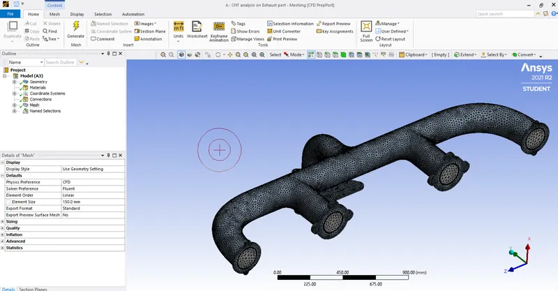
• After preparing the geometry we will mesh the solid volume and fluid volume with different mesh size.

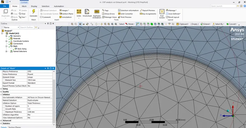
• Now we need to form an inflation layer around the boundries of fluid volume. The number of layers and its thickness will depend on the type of turbulence model that we will run on fluent.

For that we need to calculate the total thickness of the inflation layer using Y plus value.

There are 4 inlets and 1 outlet in the exhaust ports.

Cylinder port Dia = 200 mm.

Given data,

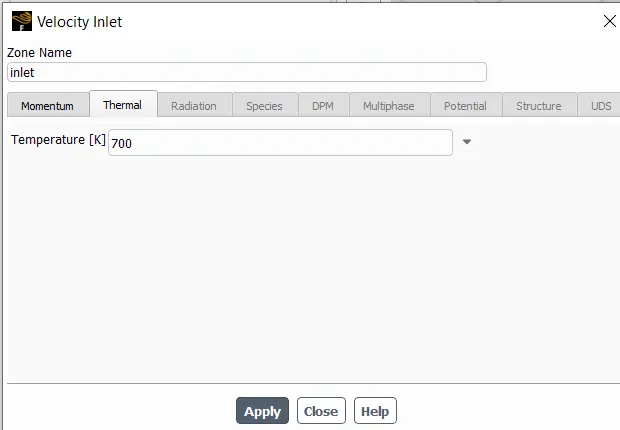
Type of fluid = Air, Inlet temperature = 700 K, Internal ref. temperature = 300K.

Density of Air = 1.225kg/m3, Dynamic Viscosity = 1.789e-5 kg/ms, Velocity of the fluid = 5 m/s.

Reynolds Number = `(rhoUL)/mu` = 68458.7

We are choosing 2 turbulence models to calculate the 2 different inflation layer heights, these are k -epsilon and k- omega.

The y plus value is different for different tutbulence model.

For k-omega turbulence model,

`Y^+ = 5` (For viscous sub layer i.e, k-omega)

For k-epsilon turbulence model,

`Y^+ = 50` (For Turbulence layer i.e, k-epsilon)

Based on the Y plus value we will calculate the first layer height and total thickness of the inflation layer for both k-omega and k-epsilon turbulence model.

Coefficient of skin friction,

`C_f = 0.058xxRe^-0.2(text(External flow))`

`C_f = 0.079xxRe^-0.25(text(Internal flow))`

As we are dealing with the fluid flow inside the exhaust port we will solve the internal flow equation.

So, `C_f = 0.0048`

Wall shear stress,

`tau_w = 0.5xxC_fxxrhoxxU^2`

`tau_w = 0.0747 N//m^2`

Frictional velocity, `U_t`

`U_t = sqrt(tau_w/rho)`

`U_t = 0.25 m//s`

Now, the first layer thickness for k-omega model where `Y^+ = 5` is,

`y = (Y^+mu)/(U_trho)`

y = 0.30mm.

Hence the total thickness of the inflation layer where no. of layers are 5 with 1.5 growth rate will be 3.96 mm.

Now, the first layer thickness for k-epsilon model where `Y^+ = 50` is

`y = (Y^+mu)/(U_trho)`

y = 2.92mm.

Hence the total thickness of the inflation layer where no. of layers are 5 with 1.5 growth rate will be 38.51 mm.

For K-Omega,

For k-epsilon,

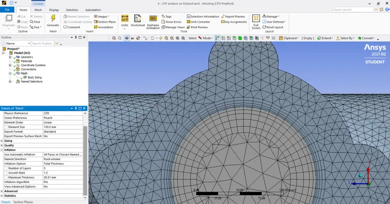
3. Problem Set-Up:

• In general settings we will choose the type of solver as pressure based. The simulation wiil be run as steady state.

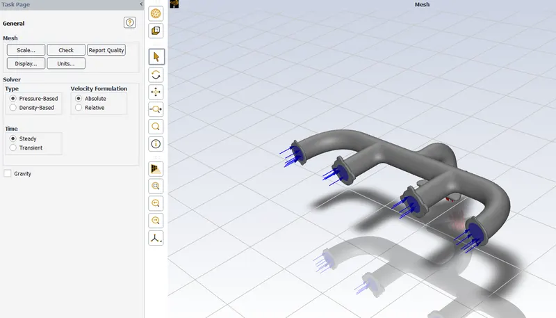
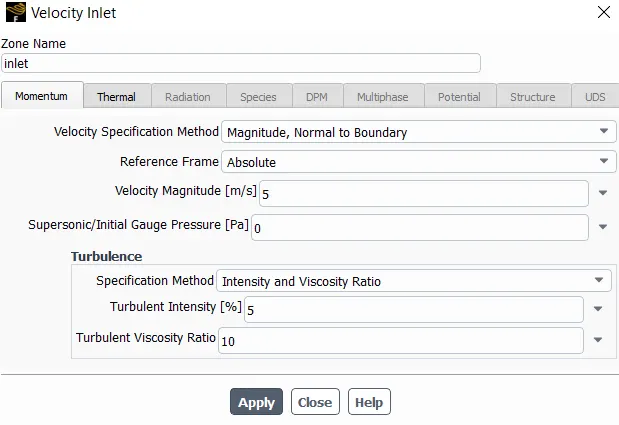
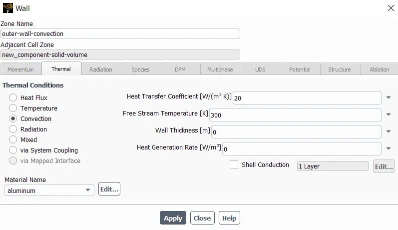
• Entering the inlet flow velocity as 5 m/s and choosing the heat transfer method as Convection with heat transfer coefficient as 20 W/m2 K

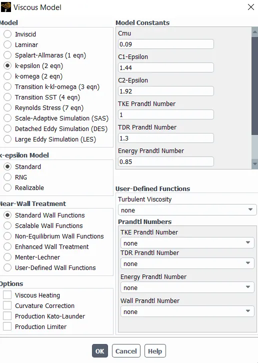
• Choosing the turbulence model.

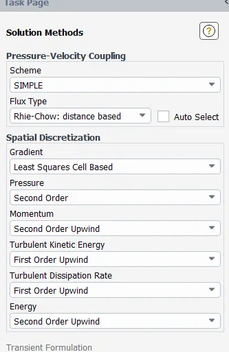
• Solution method is choosen as SIMPLE for pressure velocity coupling.

• Initialize the solver and run the simulation for 150-200 iterations.

4. Solving:

We will solve for the heat transfer coefficient analytically.

External HTC = 20 W/m2 K.

Ambient Temperature = 300 K.

Inlet Temperature = 700 K.

We need to find out the internal HTC by analytical method.

We will first calculate the Nusselt number using Diitus-Boelter equation for the internal turbulent pipe flow.

`Nu_D = 0.023xxRe_D^(4//5)xxPr^n`

`Nu_D = text(Nusselt Number)`

`Re_D = text(Reynold's Number)`

`Pr = text(Prandlt Number)`

For this case Pr = 0.71 at and n =0.4.

`Nu_D = 148.11`

Calculating the heat transfer coefficient using Nusselt number formula:

`h=(Nu_D.K)/L`

h = 17.92 W/m2 K.

We need to verifiy this value from the numerical simulation.

5. Post-Processing:

Case 1: K-epsilon model with Y plus = 50

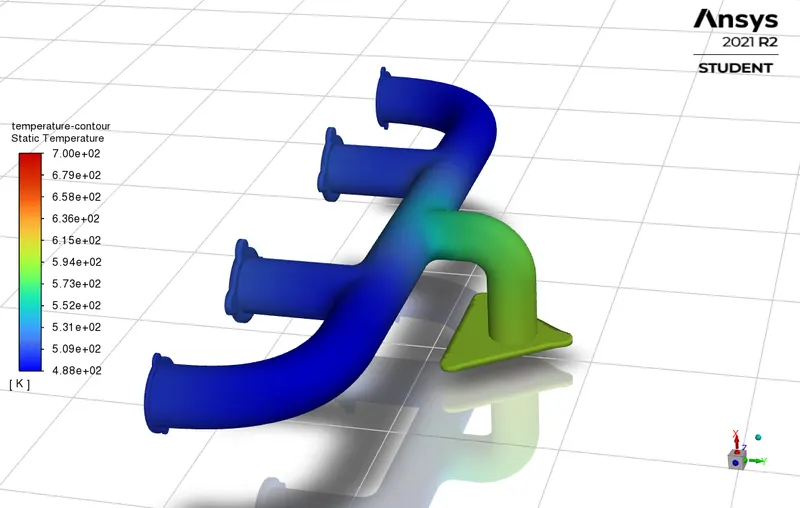
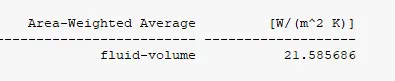
The above is the heat transfer coefficient by the ansys simulation which very close to our analytical solution.

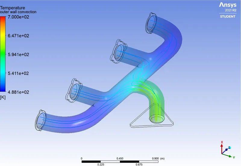
Stream line view:

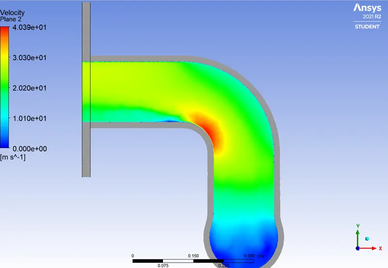
Velocity contour at the outlet:

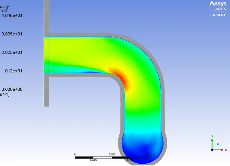
We can observe highest velocity at the red portion which is 40 m/s.

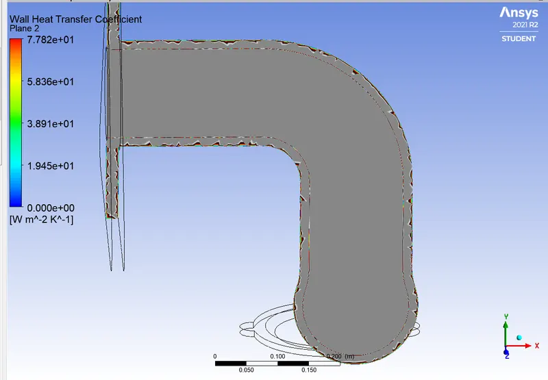
HTC contours:

Case 2: K-omega model with y plus = 5

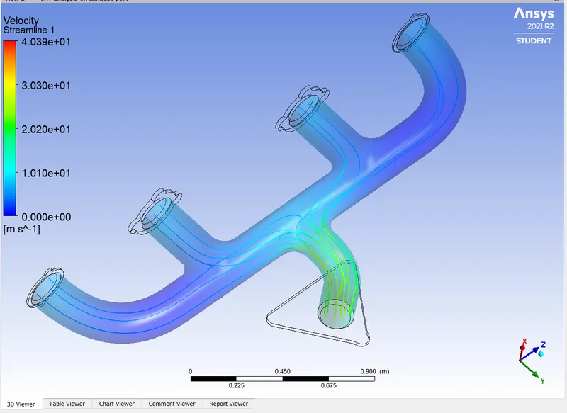
Stream line view:

Velocity contour at the outlet:

HTC contours:

• Based on the results of HTC of both the cases we can observe that k-epsilon model has calculated closest value of HTC with the analytical solution so k-epsilon model is best suited for this simulation.