Solving the steady and unsteady 2D heat conduction problem using MATLAB

MATLAB PROGRAM TO SOLVE STEADY AND UNSTEADY 2D HEAT CONDUCTION PROBLEM

Problem Statement:

Obtain temperature distribution for a thin square plate by solving 2D heat conduction equation.

To solve for 2D heat conduction equation for steady-state and unsteady-state by explicit and implicit method with given boundary conditions.

By Implicit method

Solve using different iterative solvers i.e., Jacobi, Gauss-seidel, and Successive over relaxation (SOR) for both steady and transient state heat conduction equation.

The accuracy of the solution obtained in both explicit and implicit method should be in accordance with the tolerance value mentioned.

Boundary conditions:

Top Boundary = 600 K

Bottom Boundary = 900 K

Left Boundary = 400 K

Right Boundary = 800 K

Tolerance value => error = 1e-4.

Introduction:

Numerical solution schemes are often referred to as being explicit or implicit. When a direct computation of the dependent variables can be made in terms of known quantities, the computation is said to be explicit. When the dependent variables are defined by coupled sets of equations, and either a matrix or iterative technique is needed to obtain the solution, the numerical method is said to be implicit.

Explicit Method:

When a direct computation is made for an unknown quantity in terms of known quantity. This computation is called Explicit. This method requires stability criteria which when satisfied leads to stable solution. Because of the stability criteria small time steps has to be taken to obtain stable solutions. With decrease in time step, the number of computations increases and hence the computational time required for the solution to converge is less and the accuracy of the solution is high.

Implicit Method

When a computation is made for dependent variable are defined by set of equations and a matrix is involved to find the unknown variable. This computation is called Implicit method. This method is unconditionally stable as a result, no stability criteria is required to obtain a stable results and the computational time required for the solution to converge is high and accuracy of the solution is less relative to explicit method because this method uses simultaneous equations and uses guess values as the initial values to find the approximated values. If the guess values are closer to the desired value the computation time is less. As there is no stability criteria requirement larger time steps can be used.

In order to solve for dependent variable iterative solvers are used. Iterative solvers used are

1. Jacobi iterative solver

2. Gauss seidal iterative solver

3. Successive over relaxation iterative solver.

2D Heat conduction Equation

`(delT)/(delt) = alpha*((del^2T)/(delx^2)+(del^2T)/(dely^2))`

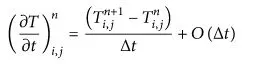
The time derivative term `(delT)/(delx)` is hyperbolic in nature which can be discretized using forward differencing scheme and the spacial derivatives are elliptical in nature which can be discretized using central differencing scheme.

Discretization of Time derivative using forward difference scheme since the time derivative is varying in time direction which can be solved by marching method.

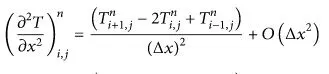
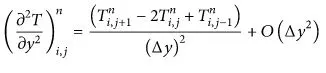
Discretization of spacial derivatives using central differencing scheme since the spacial derivatives are elliptical in nature, which uses information from neighboring points to obtain a solution. Below are the discretization for x and y spacial derivatives.

From the PDE heat conduction equation,

where n is current time step and n+1 is next time step.

i,i+1 are the neighbouring points in x direction, j,j+1 are the neighbouring points in y direction.

△x">△x is grid spacing in x direction. △y">△y is grid spacing in y direction.

Iterative Solver:

1. Jacobi iterative solver:

In this method the temperature at n+1th iteration is found using old values of the temperature defined at nth iterations. Using the approximation obtained iterations procedure it continued untill the desired accuracy of the solution is obtained.

2. Gauss Seidal iterative solver:

In this type iterative solver, temperature at n+1 iterations uses values of n+1 iterations that have already been computed. By this way old approximated values are overwritten with new approximate values for the iterations performed. Unlike jacobi, Gauss seidal require one storage vector which can be overwritten with each computation. This helps for the solution to coverge faster than the jacobi method.

3. Successive over relaxation iterative solver.

In this type of iterative solver relaxation factor is used which helps in increasing the convergence rate. It goes by the formula

`T^(n+1) = T^n * (1- omega)+omega*T(GS) or T(jacobi)`

where ω">ω is the relaxation factor . Its range is from 0<ω">ω<2

when ω">ω is between 0-1 it is called under relaxed state.

This condition is used when the temperature gradient is high and due to this condition the time step does not over shoot and helps to converge at a faster rate.

when ω">ω is between 1-2 it is called over relaxed state.

This condition is used when the temperature gradient is low and due to this condition larger time steps are used to obtain the steady state i.e., for the values to converge at faster rate.

`T^n` is the value of temperature for previous iterations

T(GS) or T(jacobi) is the temperature of value for n+1th iteration using gauss seidal or jacobi iterative solver.

Steady State 2D Heat Conduction Equation :

Steady state is where the fluid properties does not change with respect to time.

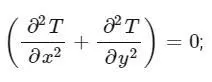
From the 2D heat conduction equation since the system is in steady state time derivative is zero and diffusivity is constant.

Hence we the equation for steady state as:-

Discretization for Steady State:

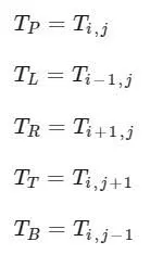
Solving for T(i,j), we get

,

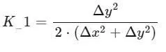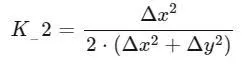
Solving the 2D Steady Heat Conduction equation implicitly.

Formula for Jacobi iterative solver:-

Formula for Gauss Seidal Iterative Solver:-

`(T_p)^(n+1) = K_1 (T_L + T_r)^(n+1)+K_2 (T_T+T_B)^(n+1)`

Formula for Successive over relaxation iterative solver:-

Transient state:

Unsteady state is where the fluid properties change with respect to time.

The formula for 2D transient heat conduction equation is :

`(delT)/(delt) = alpha*((del^2T)/(delx^2)+(del^2T)/(dely^2))`

Discretization for Unsteady State heat conduction equation:-

Solving 2D transient heat conduction equation explicitly we get,

`T_P^(n+1) = (1-2*K_1-2*K_2)*T_P^(n)+K_1(T_L+T_R)^(n)+K_2(T_T+T_B)^(n)`

`K_1 = alpha*(trianglet)/(trianglex^2)`

`K_2 = alpha*(trianglet)/(triangley^2)`

Stability Criteria:

`K_1+K_2 <= 0.5` Stability criteria for 2D heat conduction equation when solving explicitly.

Solving for 2D Transient Heat Conduction equation implicitly we get,

`T_P^(n+1) = 1/K*[T_P^(n)+K_1(T_L+T_R)^(n+1)+K_2(T_T+T_B)^(n+1) ]`

`K=1+2*K_1+2*K_2`

`K_1 = alpha*(trianglet)/(trianglex^2)`

`K_2 = alpha*(trianglet)/(triangley^2)`

here n+1 is the next time step and n is the preceeding time step.

Formula for jacobi iterative solver:-

Formula for Gauss seidal

Formula for Successive over relaxation

MATLAB Program to solve 2D steady state heat conduction using iterative solvers

% MATLAB Program to solve 2D steady state heat conduction using iterative solvers
% Steady State heat conduction
clear all;
close all;
clc;
% Initializing variables
% Specifying length of the domain, L=1
% defining space domain
Nx = 21; % number of grid points along x-axis
Ny = 21; % number of grid points along y-axis
x=linspace(0,1,Nx);
y=linspace(0,1,Ny);
% grid size
dx=1/(Nx-1);
dy=1/(Ny-1);
% Dummy error value
error = 1e9;
% tolerance
tol=1e-4;
%Coefficient obtained from the derivation for steady state equation
k=2*((1/(dx^2))+ (1/(dy^2)));

% Temperature field
T=298*ones(Nx,Ny);
T(1,:) = 600; % bottom
T(end,:)=900; % top 
T(:,1) = 400; % left 
T(:,end)=800; % right 
% Corner refining
T(1,1)=(600+400)/2;
T(1,end) = (600+800)/2;
T(end,1) = (400+900)/2;
T(end,end) = (800+900)/2;
%relaxation factor for successive over relaxation (SOR)method, for steady state heat conduction.
omega = 1.2;
% Making a copy of the initial temperature matrix
Told=T;

% Solving 2D steady state system

[xx,yy] = meshgrid(x,y);

iter_solver= input('For solver type: n 1 for Jaccobi n 2 for Gauss Siedel n 3 for SOR n'); 
tic;

%Jacobi Iteration Scheme:

if iter_solver == 1
jaccobi_iter=1;%defining iteration variable to store and display the number of iterations computed for the values to converge.

% convergence loop
while (error > tol)
    % Iteration loop
for i = 2:Nx-1
for j = 2:Ny-1
 % Calculate temperature at each grid point   
term1=(Told(i-1,j)+Told(i+1,j))/(k*(dx^2));
term2=(Told(i,j-1)+Told(i,j+1))/(k*(dy^2));
T(i,j)=term1+term2;
end
end
error = max(max(abs(Told-T))); % 2d problem so two max

%updating the temperature values for the next iteration.
Told=T;

%incrementing iter variable by 1 to display the no. of iterations taken for the solution to converge.
jaccobi_iter= jaccobi_iter +1;
end
end

% Gauss siedel iterative method
if iter_solver == 2
gs_iter=1;
while (error > tol)
for i = 2:Nx-1
for j = 2:Ny-1
term1=(T(i-1,j)+Told(i+1,j))/(k*(dx^2));
term2=(T(i,j-1)+Told(i,j+1))/(k*(dy^2));
T(i,j)=term1+term2;
end
end
error = max(max(abs(Told-T)));
Told=T;
gs_iter= gs_iter +1;
end
end

% SOR iterative solver
if iter_solver == 3
sor_iter=1;
while (error > tol)
for i = 2:Nx-1
for j = 2:Ny-1
term1=(T(i-1,j)+Told(i+1,j))/(k*(dx^2));
term2=(T(i,j-1)+Told(i,j+1))/(k*(dy^2));
T(i,j)=(1-omega)*Told(i,j)+omega*(term1+term2);
end
end
error = max(max(abs(Told-T)));
Told=T;
sor_iter= sor_iter +1;
end
end
time_required=toc;
% Plot representing the converged results
figure(1)
[C,h]=contourf(xx,yy,T);
colorbar;
colormap(jet);
clabel(C,h); %Labelling the contour plot, here C reperesents the temperature values and h rotates the temperature values as it moves

if iter_solver == 1
title_text= sprintf('Steady state heat conduction using Jacobi method n No. of Iterations: %d n Computation Time: %0.3f seconds',jaccobi_iter,time_required);
title(title_text);
saveas(figure(1), 'steady_Explicit_Jaccobi.jpeg','jpeg');
else if iter_solver == 2
title_text= sprintf('Steady state heat conduction using Gauss Siedel method n No. of Iterations: %d n Computation Time: %0.3f seconds',gs_iter,time_required);
title(title_text);
saveas(figure(1), 'steady_Explicit_Gauss_siedel.jpeg','jpeg');
else if iter_solver == 3
title_text= sprintf('Steady state heat conduction using SOR method n No. of Iterations: %d n Computation Time: %0.3f seconds',sor_iter,time_required);
title(title_text);
saveas(figure(1), 'steady_Explicit_SOR.jpeg','jpeg');
    end
    end
end
xlabel('X Length Domain');
ylabel('Y Length Domain');

Resulting plots and conclusion

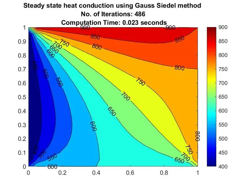
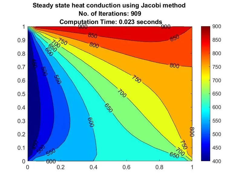
When the equation was solved using the Gauss-Siedel formula, It took 486 iterations to get converged results. This is much lower compared to the number of iterations taken to solve the same equation using the Jacobi method.(when the equation was solved using the Jacobi formula, It took 909 iterations to get converged results) Due to this the time required for computation reduces significantly compared to that of the Jacobi method. This is because the terms substituted in the discretized equation are the latest terms computed, rather than substituting the terms obtained in the previous iteration.

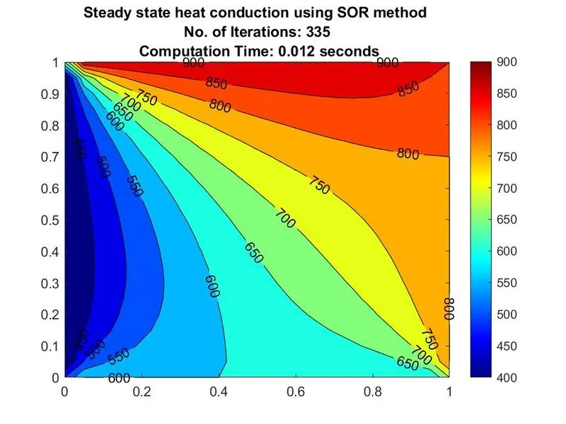
From the above result, we can see that SOR has the fastest convergence rate, followed by Gauss-Seidel and then Jacobi. The SOR method gave converged solution in 335 iterations when compared to Gauss-Seidel with 486 iterations and Jacobi with 909 iterations. Consequently, the simulation time of the SOR method was 6 times faster than the Gauss-Seidel and 11 times faster than the Jacobi.

This is because the SOR method is an optimized form of the Gauss-Seidel method which in turn, is an advanced form of the Jacobi. It scales-up the convergence rate of the Gauss-Seidel method by a factor called the relaxation factor (omega). The relaxation factor can generally take values between 0 and 2. But for this method omega>1, since we're over-relaxing. At omega=1, the SOR method is the same as the Gauss-Seidel method. At omega=0, the solution does not update at all and at omega=2, the solution blows up.

The convergence rate of SOR also depends on the choice of the relaxation factor. So, we must find an optimum value for the relaxation factor, that gives the fastest convergence rate.

MATLAB Program for 2D Transient State Heat Conduction Equation-(UnSteady State Explicit method)

% MATLAB Program  2D Transient State Heat Conduction Equation-UnSteady State Explicitly

clear all;
close all;
clc;
% Initializing variables
% Specifying length of the domain, L=1
% defining space domain
Nx =11; % number of grid points along x-axis
Ny = 11;  % number of grid points along y-axis
x=linspace(0,1,Nx);
y=linspace(0,1,Ny);
% grid size
dx=1/(Nx-1);
dy=1/(Ny-1);
alpha=1.4; % diffusivity co-efficient in the 2D heat conduction equation
dt=0.001; % time step
%%Temperature field
T=298*ones(Nx,Ny);
T(1,:) = 600; % bottom
T(end,:)=900; % top 
T(:,1) = 400; % left 
T(:,end)=800; % right 
% Corner refining
T(1,1)=(600+400)/2;
T(1,end) = (600+800)/2;
T(end,1) = (400+900)/2;
T(end,end) = (800+900)/2;
%copy T
Told=T;
%%CFL Number
CFL_num=alpha*dt/(dx^2)+ alpha*dt/(dy^2);

% Solving 2D Unsteady state system

[xx,yy] = meshgrid(x,y);
k1 = (alpha*dt)/(dx^2);
k2 = (alpha*dt)/(dy^2);
iter_solver=1; % cannot be kept inside the time loop as for every new time loop the counter will start from 1
tic;
%computing:
for nt=1:1600
 for i = 2:Nx-1
        for j = 2:Ny-1
            term1 = Told(i,j);
            term2 = k1*(Told(i-1,j)-2*Told(i,j)+Told(i+1,j));
            term3 = k2*(Told(i,j-1)-2*Told(i,j)+Told(i,j+1));
            T(i,j) = term1+term2+term3;
        end
 end
 Told = T;
 iter_solver = iter_solver+1;
end
time_required=toc;
figure(1)
[C,h]=contourf(xx,yy,T);
colorbar;
colormap(jet);
clabel(C,h);

title_text= sprintf('Unsteady state heat conduction using Explicit method n No. of Iterations: %d n Computation Time: %0.3f seconds n CFL Number=%0.2f n Time step dt = %0.4f',iter_solver,time_required,CFL_num,dt);
title(title_text);
xlabel('X Length Domain');
ylabel('Y Length Domain');
saveas(figure(1),'unsteady_explicit_dt=0.001_cfl=0.25.jpeg','jpeg');

Result plots and explanation

Matlab Program for 2D Transient State Heat Conduction Equation-(UnSteady state Implicit Method )

% MATLAB Program  2D Transient State Heat Conduction Equation-UnSteady state Implicitly
clear all;
close all;
clc;
%Initialize variables
Nx = 11; % number of grid points along x-axis
Ny = 11; % number of grid points along y-axis
x=linspace(0,1,Nx);
y=linspace(0,1,Ny);
dx=1/(Nx-1);
dy=1/(Ny-1);
%diffusivity co-efficient in the  2D heat conduction equation
alpha=1.4;
% Calculation of time step
% dt = (0.5)/((alpha/dx^2)+(alpha/dy^2));
dt=0.001;
tol=1e-4;% tolerance
%%Temperature field
T=298*ones(Nx,Ny);
T(1,:) = 600; % bottom
T(end,:)=900; % top 
T(:,1) = 400; % left 
T(:,end)=800; % right 
% Corner refining
T(1,1)=(600+400)/2;
T(1,end) = (600+800)/2;
T(end,1) = (400+900)/2;
T(end,end) = (800+900)/2;
%copy T
Told=T;
T_prev_dt = Told;
%CFL Number and omega
CFL_num=alpha*dt/(dx^2)+ alpha*dt/(dy^2);
omega=1.2; %relaxation factor for Successive over relaxation (SOR)method for transient heat conduction 

% Solving the 2D unsteady state system Implicity using iterative solvers
[xx,yy] = meshgrid(x,y);
k1 = (alpha*dt)/(dx^2);
k2 = (alpha*dt)/(dy^2);
% Input
iter_solver= input('For solver type: n 1 for Jaccobi n 2 for Gauss Siedel n 3 for SOR n'); 
jaccobi_iter=1; % cannot be kept inside the time loop as for every new time loop the counter will start from 1
gs_iter=1;
sor_iter=1;
tic;

% computing- time loop:
for nt = 1:1600
    % jocobi iterative solver
    if iter_solver == 1
    term1 = 1/(1+2*k1+2*k2);
    term2 = k1*term1;
    term3 = k2*term1;
    error = 1e9;% error outside this loop then for next time loop error will be less than tolerance and program wont procede
    while (error > tol)
       for i = 2:Nx-1
        for j = 2:Ny-1
          H = (Told(i-1,j)+Told(i+1,j));
          V = (Told(i,j-1)+Told(i,j+1));
          T(i,j) = term1*T_prev_dt(i,j)+term2*H+term3*V;
        end
       end
       error = max(max(abs(Told-T))); % 2d problem so 2 max
       Told=T;
       jaccobi_iter = jaccobi_iter +1;
    end
   end
   

% Gauss siedel iteration scheme
if iter_solver == 2
    term1 = 1/(1+2*k1+2*k2);
    term2 = k1*term1;
    term3 = k2*term1;
    error = 1e9;
    while (error > tol)
       for i = 2:Nx-1
        for j = 2:Ny-1
          H = (T(i-1,j)+Told(i+1,j));
          V = (T(i,j-1)+Told(i,j+1));
          T(i,j) = term1*T_prev_dt(i,j)+term2*H+term3*V;
        end
       end
       error = max(max(abs(Told-T))); % 2d problem so 2 max
       Told=T;
    gs_iter= gs_iter +1;
    end
end

% SOR iteration scheme
if iter_solver == 3
    term1 = 1/(1+2*k1+2*k2);
    term2 = k1*term1;
    term3 = k2*term1;
    error = 1e9;
    while (error > tol)
       for i = 2:Nx-1
        for j = 2:Ny-1
          H = (T(i-1,j)+Told(i+1,j));
          V = (T(i,j-1)+Told(i,j+1));
          T(i,j) =(1-omega)*Told(i,j)+ omega*(term1*T_prev_dt(i,j)+term2*H+term3*V);
        end
       end
       error = max(max(abs(Told-T))); % 2d problem so 2 max
       Told=T;
    sor_iter= sor_iter +1;
    end
end
T_prev_dt=T;
end
time_required=toc;
figure(1)
[C,h]=contourf(xx,yy,T);
colorbar;
colormap(jet);
clabel(C,h);

if iter_solver == 1
title_text= sprintf('unsteady state heat conduction using Jacobi method n No. of Iterations: %d n Computation Time: %0.3f seconds n CFL number = %0.3f & dt = %0.4f',jaccobi_iter,time_required,CFL_num, dt);
title(title_text);
saveas(figure(1), 'unsteady_Implict_Jaccobi_dt=0.001_cfl=0.28.jpeg','jpeg');
else if iter_solver == 2
title_text= sprintf('unsteady state heat conduction using Gauss Siedel method n No. of Iterations: %d n Computation Time: %0.3f seconds n CFL number = %0.3f & dt = %0.4f',gs_iter,time_required,CFL_num,dt);
title(title_text);
saveas(figure(1), 'unsteady_Implict_Gauss_Siede_dt=0.001_cfl=0.28.jpeg','jpeg');
else if iter_solver == 3
title_text= sprintf('unsteady state heat conduction using SOR method n No. of Iterations: %d n Computation Time: %0.3f seconds n CFL number = %0.3f & dt = %0.4f',sor_iter,time_required,CFL_num, dt);
title(title_text);
saveas(figure(1), 'unsteady_Implict_SOR_dt=0.001_cfl=0.28.jpeg','jpeg');
    end
    end
end

xlabel('X Length Domain');
ylabel('Y Length Domain');

Result plots and Explanation

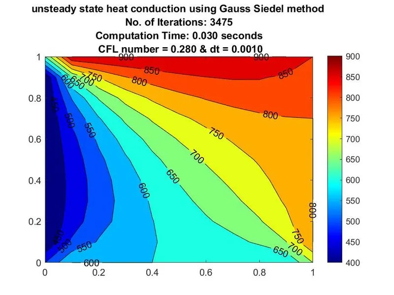
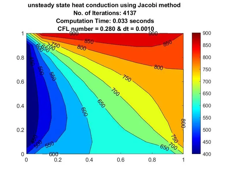
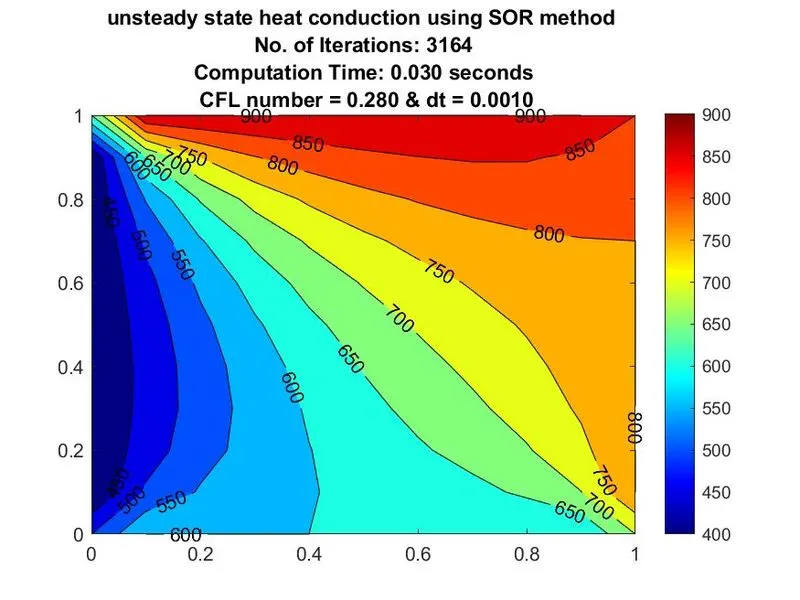
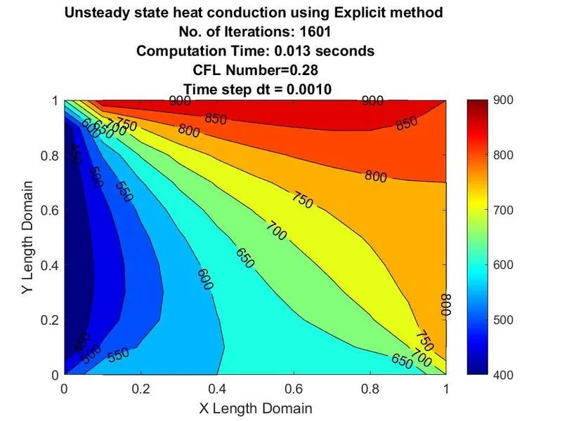
From the above results, we can see that the explicit method gives the solution fastest. This is because it does not require guess values and iterations for convergence as the explicit solution is solely based on the previous state values which had already been computed.

The implicit method requires guess values and iterations for convergence as it is also based on the future state values, which are not known at the time of computation. It checks convergence for each time step. This causes a delay in the simulation.

From the above plots, it can be found that the explicit scheme is the fastest to solve the transient state 2D heat equation because we're not bothered about iterations and convergence. The scheme uses already defined previous state values to compute present state values. So, there is no need for guess values and convergence criteria. However, the explicit scheme is strictly governed by the CFL stability condition. For a scheme to be stable,

where alpha is called the thermal diffusivity and is taken as 1.4 in this case for a faster solution.

This is a huge disadvantage for the explicit scheme because we must use extremely small values of dt as compared to dx for the solution to be stable, which means longer computational time. The above explicit solution is stable as the CFL number is 0.28, which is well below 0.5. And the solution blew for dt=1e-3 (CFL = 0.3) as the Courant's number approaches the limit.

The implicit schemes are slower and more complicated than the explicit scheme, since we're using guess values and iterating for convergence in each time step. However, they are unconditionally stable for any choice of dt with respect to dx. They offer better stability and larger time step sizes.

Below Table gives the number of iterations required by iterative solvers to converge.

Steady State Heat Conduction Equation
Iterative Solver	No. of iterations
Jacobi	909
Gauss Seidal	486
Successive over Relaxation	335

Unsteady State Heat Conduction Equation.
Iterative Solver	No. of iterations
Jacobi	4137
Gauss Seidal	3475
Successive over Relaxation	3164

Conclusion

• Steady-state conduction is the form of conduction that happens when the temperature difference driving the conduction is constant with respect to time. On the other hand, in transient-state condition, the temperature at the boundaries changes with time, and eventually reach a steady state if the temperature is not changed further.
• If the error term obtained is below the tolerance value, the solution is said to be converged. In the above problem which is solved in steady and unsteady-state conditions, we obtain an error term below the tolerance value(1e-4) for each case, hence the solution is converged.
• In the steady-state analysis and transient-state analysis using the implicit method, the solution is obtained using three methods, namely, Jacobi(J), Gauss-Seidel(GS), and successive over-relaxation(SOR) method. Out of these three methods, the third method, SOR converges to the solution with a lower number of iterations compared to the other two methods, provided that the value of omega is appropriate. The Jacobi method in both cases converges to the solution with the highest number of iterations compared to the other two methods.
• From this, we can conclude that the successive over-relaxation method is the most effective method since it converges the solution for a lesser number of iterations and hence less time is taken for solving compared to Jacobi and Gauss-Seidel method. This largely depends on the value of omega, if an appropriate value is chosen, then the solution converges faster, else the solution may take longer to converge.

• Implicit method can be used to problems when converged results are needed in less computation time as they are unconditionally stable. With increases in time step size the convergence rate is increased which leads to steady state with less no. of iterations.
• Explicit method results time accurate solutions as it is governed by stability criteria when not satisfied it leads to unstable solution and requires more iterations to attain steady state.
  
• But in the code provided above time step size remains constant which is calculated with respect to the stability criteria. Hence for this time step size the explicit scheme leads to faster convergent rate and as the time step size is small the number of iterations increases for implicit scheme which results slower convergence rate.