Week 3 - Taylor table method and Matlab code

Introduction:

Taylor Series

Taylor series of a function of infinite number of terms that are expressed in their function derivatives at a single point. The partial sum formed by the first n terms of a taylor series is a polynomial of degree n is called a nth taylor polynomial. The accuracy of the taylor polynomial is increased by increasing the n terms in taylor series. Taylor's Theorem gives a quantitative estimates of the error introduced by the use of such approximations. If the solution of function is analytic at point x and is equal to taylor series at some open interval then the function is analytic at every point of the interval.

Taylors Series.

Taylor Series: Represents a function as an infinite sum of terms that are calculated from the values of function derivative at a single point

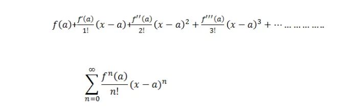
where n! is factorial of n and nth derivative of f is evaluated at a. When a= 0 the above series is called a Maclaurin series.

where y is the function of x.

Taylors Table

Taylors table is calculated to reduce the complexity of finding the solution of desired accuracy using taylors series.

Right sided difference Taylors table

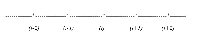
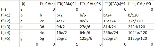
Formula of Skewed right sided difference scheme:

d`(del^2y)/(delx^2)=(y(1)*f(x)+y(2)*f(x+dx)+y(3)*f(x+2.dx)+y(4)*f(x+3.dx)+y(5)*f(x+4dx)+y(6)*f(x+5*dx))/(dx^2)`

where `f(x)=e^x*cos(x)`

Y is matrix of containing coefficients from the taylors table whose values are

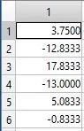
Central Difference Taylors table

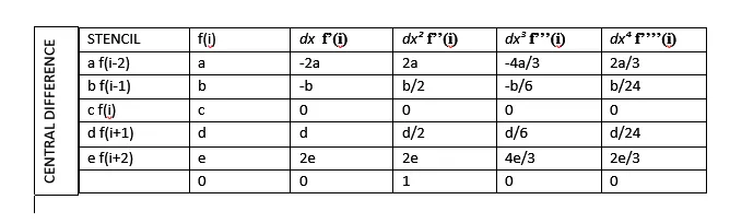
Formula for Central difference approximation using taylors table:

`(del^2y)/(delx^2)=(x(1)*f(x-2dx)+x(2)*f(x-dx)+x(3).f(x)+x(4)*f(x+dx)+x(5)*f(x+2.dx))/(dx^2)`

where `f(x)=e^x*cos(x)`

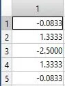
X is matrix of containing coefficients from the taylors table whose values are

Skewed left sided difference taylors table

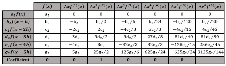
Formula of Skewed left sided difference scheme:

`(del^2y)/(delx^2)=(z(1)*f(x)+z(2)*f(x-dx)+z(3)*f(x-2.dx)+z(4)*f(x-3.dx)+z(5)*f(x-4dx)+z(6)*f(x-5*dx))/(dx^2)`

where `f(x)=e^x*cos(x)`

Z is matrix of containing coefficients from the taylors table whose values are

Proof that the derived equation is 4th order accurate:

Formula :

p=n-q+1 for central difference scheme

where p is the order of accuracy,
n is number of nodes,
q is order of derivative.

p = 5-2+1

p = 4 which represent 4th order accurate of 2nd order derivative.

p=n-q for skewed difference scheme

where p is the order of accuracy,
n is number of nodes,
q is order of derivative.

p = 6-2.

p = 4 which represent 4th order accurate fof 2nd order derivative.

Logic:

The co-efficients of the taylors series terms should be calculated.
Substitution of the taylors series in formulas for approximation methods
Calculation of error of the approximation values by comparing it with the analytical values.
Plot the graph of dx vs error to understand the variation of error with value of step length dx.

MATLAB PROGRAM TO FIND COEFFICIENT FROM TAYLOR TABLE

clear all
close all
clc
 
  % Taylor_table_coeffecients
  % central difference scheme requires information from both sides ( symmetric)
  % To obtain the 4th order approximated second-order derivative, we need information from 5 equally distributed neighboring points 
  
   [A]= [ 1 1 1 1 1; 
          -2  -1 0 1 2; 
          2  1/2 0 1/2 2; 
         -8/6 -1/6  0 1/6 8/6;
         16/24 1/24 0 1/24 16/24];
        
   [B] = [0;0;1;0;0:0];
   
   %solving matrix A&B to find constants
   X = linsolve(A,B)
   
   % skewed right-sided difference scheme requires information on the right side
   
   [C]= [ 1 1 1 1 1 1; 
          0 1 2 3 4 5; 
          0 1/2 2 9/2 8 12.5; 
          0 1/6 4/3 9/2 32/3 125/6;
         0 1/24 2/3 27/8 32/3 625/24;
         0 1/120 32/120 243/120 1024/120 3125/120 ];
        
   [D] = [0;0;1;0;0;0];
   
   %solving matrix C&D to find constants
   Y = linsolve(C,D)
   
   % skewed left-sided difference scheme requires information on the right side
   
   [E]= [1 1 1 1 1 1; 
         0 -1 -2 -3 -4 -5; 
         0 1/2 2 9/2 8 12.5; 
         0 -1/6 -4/3 -9/2 -32/3 -125/6;
         0 1/24 2/3 27/8 32/3 625/24;
         0 -1/120 -32/120 -243/120 -1024/120 -3125/120];
        
   [F] = [0;0;1;0;0;0];
   
   %solving matrix C&D to find constants
   Z = linsolve(E,F)
   
   % sum of coeffecinets should be zero
   % check
   check_X = X(1)+X(2)+X(3)+X(4)+X(5);
   check_central_difference = rats(check_X);
   check_Y = Y(1)+Y(2)+Y(3)+Y(4)+Y(5);
   check_skewed_right = rats(check_Y);
   check_Z = Z(1)+Z(2)+Z(3)+Z(4)+Z(5);
   check_skewed_left = rats(check_Z);

MAIN PROGRAM

clear all
close all
clc
   % Taylor_table_test
   % analytical function f' = exp(x)*cos(x)
   % f'' = -2*exp(x)*sin(x)
   x = pi/3;
   dx = linspace(pi/10,pi/400,100);
   
   analytical_function = exp(x)*cos(x);
   analytical_derivative = -2*exp(x)*sin(x);
   
   
   for i = 1:length(dx)
     
   a(i) = (exp(x-(5*dx(i)))*cos(x-(5*dx(i))));
   b(i) =  (exp(x-(4*dx(i)))*cos(x-(4*dx(i))));
   c(i) =  (exp(x-(3*dx(i)))*cos(x-(3*dx(i))));
   d(i) =  (exp(x-(2*dx(i)))*cos(x-(2*dx(i))));
   e(i) =  (exp(x-dx(i))*cos(x-dx(i)));
   f(i) =   exp(x)*cos(x);
   g(i) =   (exp(x+dx(i))*cos(x+dx(i)));
   h(i) =   (exp(x+(2*dx(i)))*cos(x+(2*dx(i))));
   j(i) =   (exp(x+(3*dx(i)))*cos(x+(3*dx(i))));
   k(i) =   (exp(x+(4*dx(i)))*cos(x+(4*dx(i))));
   l(i) =   (exp(x+(5*dx(i)))*cos(x+(5*dx(i))));
   
   fourth_order_second_derivative_skewed_right(i) = (45*(f(i))-154*(g(i))+214*(h(i))-156*(j(i))+61*(k(i))-10*(l(i)))/(12*(dx(i)^2));
   
   fourth_order_second_derivative_skewed_left(i) = (45*(f(i))-154*(e(i))+214*(d(i))-156*(c(i))+61*(b(i))-10*(a(i)))/(12*(dx(i)^2));
   
   fourth_order_second_derivative_central_difference(i) = (-1*(d(i))+16*(e(i))-30*(f(i))+16*(g(i))-(h(i)))/(12*(dx(i)^2));
  
   
   fourth_order_skewed_right_error(i) = abs(fourth_order_second_derivative_skewed_right(i)- analytical_derivative);
   
   fourth_order_skewed_left_error(i) = abs(fourth_order_second_derivative_skewed_left(i)- analytical_derivative);
   
   fourth_order_central_difference_error(i) = abs(fourth_order_second_derivative_central_difference(i)- analytical_derivative);
   
   
   
   end
   
   %Error comparsion between the above three schemes
   figure(1)
   loglog(dx,fourth_order_skewed_right_error, '-kd', 'markerfacecolor','r','markersize',10,'linewidth',2)
   hold on
   loglog(dx,fourth_order_skewed_left_error,'-ko', 'markerfacecolor','b','markersize',10,'linewidth',2)
   hold on
   loglog(dx,fourth_order_central_difference_error,'-ks', 'markerfacecolor','g','markersize',10,'linewidth',2)
   hold on
   legend('skewed right sided difference scheme','skewed left sided difference scheme','central difference scheme','location','northwest');
   xlabel('dx')
   ylabel('absolute error')
   title( ' Comparision of error between different schemes of 4th order approximations of the second-order derivative')

RESULTS AND OBSERVATION

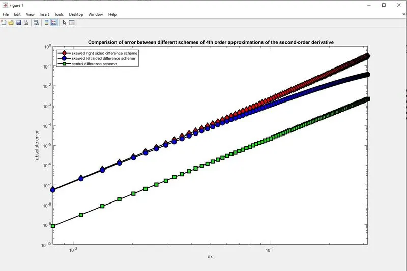
FDS and BDS require information on the right and left neighboring points respectively. In FDS and BDS it solves the equation with 1st order approximation with 1st order derivative and the central differencing scheme solve the equation with 2nd order approximation with 1st order derivative both are using same two-point information but CDS provides more accurate results.

1. Skewed right side difference gives the maximum error at almost every point of the dx.
2. The central difference gives the lowest error and is consistent throughout the range of dx.
3. Skewed left is quite unstable as at some point it gives a lower error value than the central difference and at some point it becomes almost equal to SRS difference.
4. On dropping the value of dx, the value of error also decreases. As they all are a fourth-order approximation, the slope of the curve is almost similar tp each other.

Q2. why a skewed scheme is useful? What can a skewed scheme do that a CD scheme cannot?

The skewed scheme works well when no of points available on one side of the grid. Indeed, for calculating corner node with higher approximations we need skewed scheme at this point for this type no longer central scheme useful. for example, in a pipe flow at the upstream side can be used to calculate the downstream side flow behavior in the skewed scheme, but in the central scheme we need to depend on both sides, not every time information is available for both sides of the ith point.

As we know that these schemes are used to calculate the derivative of the function at a certain point like in this case it is `(pi)/3`. This point lies somewhere between but not the endpoint/boundary points.

When it comes to calculating the derivative at boundary points, the central difference can't be used. This is because the in central difference data from both sides of the curve is required but at the boundary only one side is available.

To calculate the derivate at boundary points, Skewed right side difference and Skewed left side difference can be used. Sometimes forward difference and the backward difference can also be used but due to lack of higher-order terms, the higher-order approximation can not be calculated.

Although the Central difference gives the least error but when it comes to boundary points, due to lack of neighboring information, skewed schemes are used and gives stable results.