Week 9 - FVM Literature Review
Finite Volume Method(FVM)
It is one of the methods of solving partial differential equations by converting them into algebraic equations and then solving them using iterative solvers or the matrix inversion method. In this method, volume integration of the partial differential equation is converted into surface integral using the gauss divergence theorem.
The resulting equations are solved for the flux terms. The flux entering the through control volume is equal to the flux leaving the control volume. Hence the resulting solution is always conserved, another advantage is that this method can be applied to an unstructured mesh.
For example, Solving for 1D linear Heat conduction equation using Central Difference scheme.
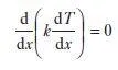
Governing equation for 1D linear Heat conduction equation
The volume considered is divided into 5 control volumes as shown in the figure.

In the above figure `T_A and T_B` are the boundary values of the temperature.
The temperature values are available at the nodal values hence the integration of the governing equation over the control volume which results in the fluxes of the control volume faces. Here linear interpolation scheme is used as the discretization scheme which when applied results in the following equation.

which when rearranged and simplified gives
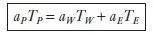
where
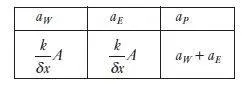
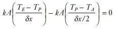
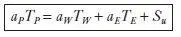
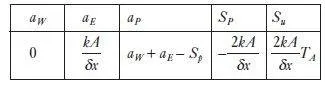
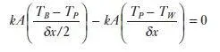
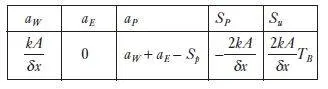
When solving for the 1st and 5th nodal points special attention to be given as the distance between the nodal points is changed. Which is solved as
Solving for 1st Nodal points

Solving for 5th nodal point

The major difference between FVM and FDM are:
1. Since the governing equations are conservative in nature, FVM solves the governing partial differential equations over the control volume using the gauss divergence theorem which results in conservative equations.
2. Major advantage of the FVM is that it only needs to calculate the flux variables at the volume boundaries. This can be applied to all non-linear conservative governing equations. Hence this method is widely used in CFD applications.
3. The accuracy of the finite volume method for the area of interest can be increased by using finer mesh in that area.
4. It is difficult to obtain higher-order schemes in the finite volume method when compared to the finite difference method.
5. The accuracy and stability of the solution in the finite difference method depend on the initial and boundary conditions.
Most of the flow problems in CFD consist of convection and diffusion terms in which a linear interpolation scheme that is a Central difference scheme can not be used as it would give erroneous results because of the presence of large oscillations if a finer mesh is not used. Because of this, there was a need to use other interpolation schemes. Irrespective of the differencing methods used numerical results obtained are close to the exact solution of the governing equation when the number of cells in large but are results of the discretization scheme will be physically realistic when it has certain fundamental properties which are:
1. Conservativeness
The integration of the convection-diffusion equation over a finite number of control volumes results in discretized conservative equations involving fluxes. For the equations to be conversed the flux leaving the control volume face should be equal to flux entering the control volume face.
2. Boundedness.
This property means that an increase in the flow variable at one node will result in an increase of the flow variables in the neighboring nodes. If the discretization scheme does not satisfy the conditions for boundedness then the solution does not converge, even if it converges it contains wiggles.
The conditions for boundedness are :
a) All coefficients of the discretized equations should have the same sign (positive).
b) The resulting matrix from the discretization should be diagonally dominant.
3. Transportiveness.
Transportiveness defines the relationship between the directionality of influencing and the flow direction and magnitude of the Peclet number.
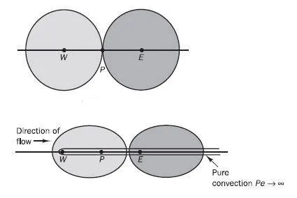
In the first figure, it is a pure diffusion process hence point P is influenced by both point W and E. Whereas in the second figure as Pe increases the flow is convection dominated and the shape changes to elliptical and shifts in the direction of the flow. In this figure, the point is influenced by point W only since the direction of the flow is in the positive x-direction. Point P will be influenced by Point E if the flow is in the negative x-direction.
Different differencing schemes are:
1.Central Differencing Scheme
The CDM uses consistent expressions to evaluate convective and diffusive fluxed at the control volume faces. Hence this is conserved.
This scheme is not bounded as it violates the boundedness conditions and leads to physically impossible solutions.
Since the scheme uses neighboring points to calculate the convective diffusive fluxes it does not recognize the direction of the flow. It does not possess the transportiveness at high Pe.
2. Upwind Differencing scheme.
This scheme uses consistent expressions to calculate the fluxes through cell faces therefore it is conserved.
The coefficients of the discretized equation are always positive and satisfy the requirements for boundedness.
The scheme accounts for the direction of the flow so it possesses transportiveness property.
3. Hybrid Differencing scheme
The hybrid differencing scheme is a mix of the upwind and central differencing scheme. It switches to the upwind differencing scheme when the central differencing scheme produces inaccurate results at a high Pe number. The scheme is fully conservative and since the coefficients are always positive it is unconditionally bounded. It also satisfies the transportiveness by using an upwind differencing scheme for large values of Pe number.
Flux limiters:
Oscillations are created when discretizing non-linear governing equations which results in unrealistic values for flow variables. In order for the interpolation scheme to result realistic value limits are introduced. These limits are called flux limiters. They limit the solution gradient near shocks or discontinuous. The name flux limiter because the limiter acts on system fluxes.