Week 3 - Solving second order ODEs

Solving Second order ODE of motion of simple pendulum using MATLAB, also to create a simulation showing the motion of simple pendulum

• Simple Pendulum

A simple pendulum consists of a ball (point-mass) m hanging from a (massless) string of length L and fixed at a pivot point P. When displaced to an initial angle and released, the pendulum will swing back and forth with periodic motion. By applying Newton's secont law for rotational systems, the equation of motion for the pendulum may be obtained

ORDINARY DIFFERENTIAL EQUATION (ODE) :-

An ordinary differential equation (also abbreviated as ODE), in Mathematics, is an equation which consists of one or more functions of one independent variable along with their derivatives.

In Engineering, ODE is used to describe the transient behavior of a system. A simple example is a pendulum

The way the pendulum moves depends on the Newton's second law. When this law is written down, we get a second order Ordinary Differential Equation that describes the position of the "ball" w.r.t time.

Similarly, there are hundreds of ODEs that describe key phenomena and if you have the ability to solve these equations then you will be able to simulate any of these systems.

The second-order ODE for simple pendulum is represented as,

`(del^2theta)/(del t^2)+ (b/m)*(deltheta)/(delt)+g/l*sintheta=0`

where; b = damping coefficient = 0.05,

m = mass of ball = 1 kg,

g = acceleration due to gravity = 9.81 m/s^2,

l = length of the string = 1 metre.

we are converting the second-order ODE into two first-order ODEs

let's take `theta=theta1`

so, `(deltheta)/(delt)=(deltheta1)/(delt)=theta2` ----->[1]

now , `(del^2theta)/(delt^2) = (del^2theta1)/(delt^2) = (del)/(del t) (deltheta1)/(delt) = (deltheta2)/(delt) ---->[2]`

Now 2nd order ODE becomes, ( By applying equation 1 & 2 )

`(del theta2)/(delt)+(b/m)*(deltheta1)/(delt)+g/l*sintheta1=0`

`(del theta2)/(delt)+(b/m)*(theta2)+g/l*sintheta1=0`

`(del theta2)/(delt)`= `-(b/m)*(theta2)-g/l*sintheta1`

so we split the second-order ODE of motion of simple pendulum into two first-order ODEs as mentioned below,

`(deltheta1)/(delt)=theta2` ----> (first ODE )

`(deltheta2)/(delt)= -b/mtheta2-g/lsintheta1` ---> (second ODE )

Now we solve these ODEs using 'ode45' function in matlab.

Ode45 is a function in matlab that solves ordinary or partial differential equations using a numerical method. The numerical method in question here is the 4th order Runge Kutta method.

How ode45 works:

The function ode45 takes 3 inputs. The 3 inputs are the function to be integrated, the time span and the initial conditions.

Syntax

where tspan = [t0 tf], integrates the system of differential equations y′=f(t,y) from t0 to tf with initial conditions y0. Each row in the solution array y corresponds to a value returned in column vector t.

so we have to create an ode function ('ode_fun') separately and call it during the run of 'ode45' function in the main program.

Program for the 'ode_function'

function [dtheta_dt]=ode_fun(t,theta,b,g,l,m)

theta1 =theta(1);
theta2=theta(2);
dtheta1_dt=theta2; % 1st ODE
dtheta2_dt=-(b/m)*theta2-(g/l)*sin(theta1); % 2nd ODE
dtheta_dt =[dtheta1_dt;dtheta2_dt]

end

Program to solve Second order ODE of motion of simple pendulum using MATLAB, also to create a simulation showing the motion of simple pendulum

 %     PROGRAM TO SOLVE SECOND ORDER ODE REPRESENTING EQUATION OF MOTION OF A SIMPLE PENDULUM

close all
clear all
clc

%step 1: input values

b=0.05; % Damping Coefficient

g=9.81; % acceleration due to gravity, m/s^2

l=1; % length of the pendulum , m

m=1 ; %mass of ball, kg

%step 2:Initial condition for displacement and angular velocity

theta_0=[0;3]; % angular displacement=0,angular velocity= 3 rad/sec at time t=0

%step 3: time span
t_span = linspace(0,20,500); % pendulum moves from 0 to 20 sec with 500 equal intervals

%step 4: Solving ODE

% call ode_fun function
% ode45 gives result in rad and rad/s.

% ODE Solver, [t,y] = ode45(odefun,tspan,y0)

[t,result]=ode45(@(t,theta)ode_fun(t,theta,b,g,l,m),t_span,theta_0);

%step 5 :plotting 

figure(1)
plot(t,result(:,1))% Plotting displacement values in a column matrix
hold on
plot(t,result(:,2))% plotting angular velocity valuesin a column matrix
title('For Simple Pendulum')
xlabel('Time in sec')
ylabel('Angular Velocity(rad/s) / Displacement(rad)')
legend('Displacement','Angular velocity')

%step 6 : simulating motion of simple pendulum

amplitude=result(:,1); %store amplitude values in separate matrix for loop
ct=1;
for i=1:length(amplitude)
    angle=amplitude(i);
    figure(2)
    title('Simple Pendulum')
    
    %fix point of pendulum
    
    x0=0;
    y0=0;
    
    %another end of pendulum/cordinate of mass ball 
    
    x1=l*sin(angle);
    y1=-l*cos(angle);
   
    % plot
    
    plot([-1.1 1.1],[0 0],'linewidth',2); %ceiling line
    
    hold on 
    
    plot([x0 x1],[y0 y1],'color','g','linewidth',2)% pendulum string
    
    plot(x1,y1,'o','markers',20,'markerfacecolor','r') % mass ball
    
    hold off %removing previous position
    
    grid on 
    axis([-1.5 1.5 -1.5 0.5])
    pause(0.03)
    M(ct) = getframe(gcf);
    ct = ct+1;
end

%step 7: making movie
movie(M)
videofile = VideoWriter('simple_pendulum.avi','uncompressed avi');
open(videofile)
writeVideo(videofile,M)
close(videofile)

Procedure

1) we started the program with ' clear all', 'close all', 'clc' functions

"clear" function removes items ( variables, scripts and functions, class definition etc. ) from workspace and freeing up system memory.

"close all" closes all figures whose handles are visible. A figure handle is hidden if the HandleVisibility property is set to 'callback' or 'off

"clc" clears all the text from the Command Window, resulting in a clear screen.

2 ) then we define input values

b=0.05; % Damping Coefficient

g=9.81; % acceleration due to gravity, m/s^2

l=1; % length of the pendulum , m

m=1 ; %mass of ball, kg

3 ) then we define initial condition and time span

Initial condition for displacement and angular velocity

theta_0=[0;3]; % angular displacement=0,angular velocity= 3 rad/sec at time t=0

time span

t_span = linspace(0,20,500); % pendulum moves from 0 to 20 sec with 500 equal intervals

4 )Then we have to solve the ODEs using "ode45" function, by calling the "ode_function" we created before.

[t,result]=ode45(@(t,theta)ode_fun(t,theta,b,g,l,m),t_span,theta_0);

results will be stored in [t,result] matrix.

5) Now we are plotting displacement and angular velocity values obtained by solving ODEs, using plotting command

figure(1)
plot(t,result(:,1)) % Plotting displacement values in a column matrix
hold on
plot(t,result(:,2)) % plotting angular velocity valuesin a column matrix
title('For Simple Pendulum')
xlabel('Time in sec')
ylabel('Angular Velocity(rad/s) / Displacement(rad)')
legend('Displacement','Angular velocity')

6 ) In the next step in order to simulate the motion of simple pendulum we are using ''For loop" and we are creating lines between fixed position of pendulum and each position of displacement values obtained in the result. and saved in another figure.

amplitude=result(:,1); %store amplitude values in separate matrix for loop
ct=1;
for i=1:length(amplitude)
angle=amplitude(i);
figure(2)
title('Simple Pendulum')

%fix point of pendulum

x0=0;
y0=0;

%another end of pendulum/cordinate of mass ball

x1=l*sin(angle);
y1=-l*cos(angle);

% plot

plot([-1.1 1.1],[0 0],'linewidth',2); %ceiling line

hold on

plot([x0 x1],[y0 y1],'color','g','linewidth',2)% pendulum string

plot(x1,y1,'o','markers',20,'markerfacecolor','r') % mass ball --> in this step we are creating circle in order to represent mass ball, by using "markers" command

hold off %removing previous position

grid on
axis([-1.5 1.5 -1.5 0.5])
pause(0.03)
M(ct) = getframe(gcf);
ct = ct+1;
end

7 ) Finally creating movie from all the frames collected in 'M', using "VideoWriter" function

movie(M)
videofile = VideoWriter('simple_pendulum.avi','uncompressed avi');
open(videofile)
writeVideo(videofile,M)
close(videofile)

Errors occured during Programing

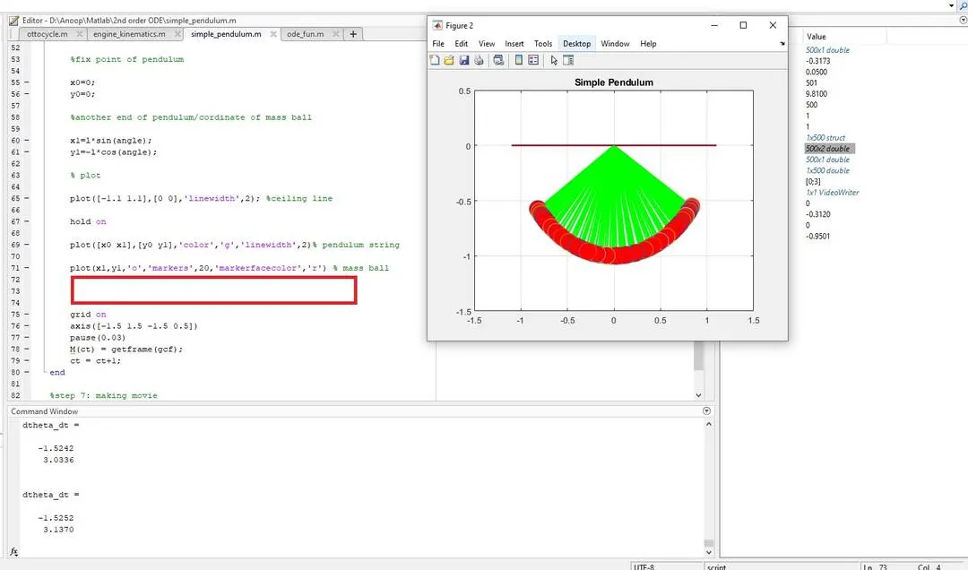
as shown in figure above forgot to give "hold off" command after plotting figure2, so while animating it's showing frames in each and every position.

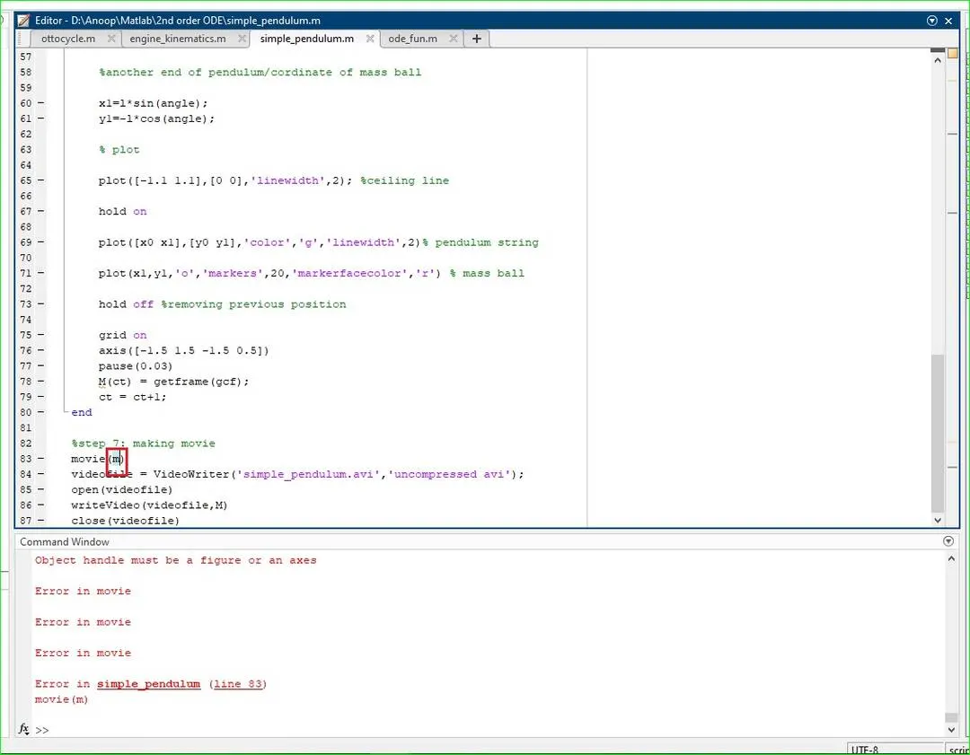
in movie command while typing 'M' was typed in lower case instead of upper case.

Results

solved 2nd order ODE for the motion of simple pendulum and displacement and angular velocty values obtained during the time span is plotted in a grapg shown below.

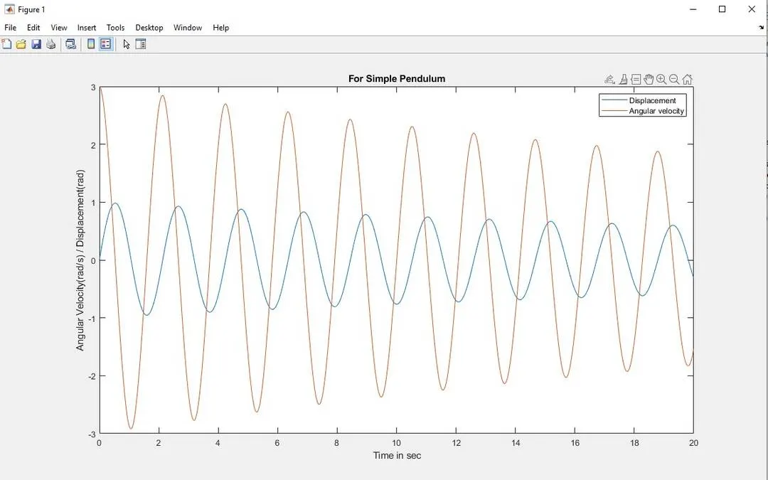
also simulation showing motion of simple pendulum is shown below