Rankine cycle Simulator using MATLAB
Rankine cycle Simulator using MATLAB
Aim
- Create a Rankine Cycle Simulator using OCTAVE/MATLAB.
- Write code to calculate the state points of the Rankine Cycle based on user inputs.
- Then, plot the corresponding T-s and h-s plots for the given set of inputs.
- Calculate Net Work output & Back work Ratio, Thermal efficiency of the cycle.
RANKINE CYCLE:
It is the basic operating cycle for all power plants where a working fluid is continuously changing its phase from liquid to vapor and vice-versa. It is well known as modified Carnot cycle , where condensation process is continued until the steam condensed in to water.
Rankine cycle is also defined: if the working fluid in a vapor cycle passes through various components of the power plant without irreversibility and frictional pressure drop, then the cycle is called as Ideal Rankine Cycle.
Many of the impracticalities associated with the Carnot cycle can be eliminated by superheating the steam in the boiler and condensing it completely in the condenser. The cycle that results is the Rankine cycle, which is the ideal cycle for vapor power plants. The ideal Rankine cycle does not involve any internal irreversibility. The below picture depicts Rankine cycle.
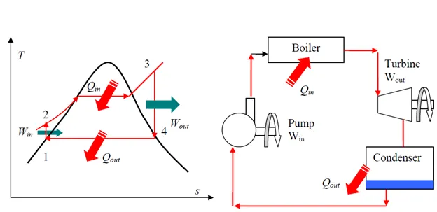
PROCESS_1-2 ISENTROPIC COMPRESSION: Water enters the pump as state 1 as saturated liquid and is compressed isentropically to the operating pressure of the boiler.
PROCESS_2-3 CONST PRESSURE HEAT ADDITION: Saturated water enters the boiler and leaves it as superheated vapor at state 3.
PROCESS_3-4 ISENTROPIC EXPANSION: Superheated vapor expands isentropically in turbine and produces work.
PROCESS_4-1 CONST PRESSURE HEAT REJECTION: High quality steam is condensed in the condenser.
Energy Analysis of the Ideal Rankine Cycle: All four components of the Rankine cycle are steady-state steady-flow devices. The potential and kinetic energy effects can be neglected. The first law per unit mass of steam can be written as:
steady-flow energy equation:

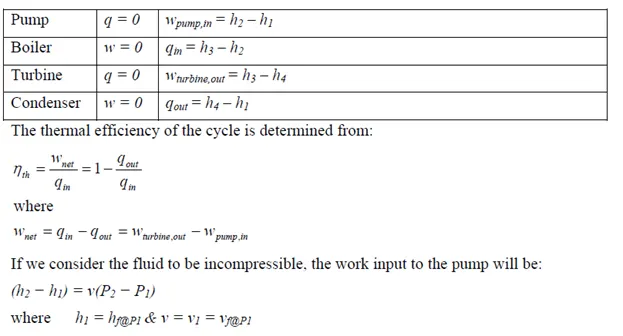
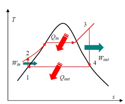
The thermal efficiency can be interpreted as the ratio of the area enclosed by the cycle on a T-s diagram to the area under the heat-addition process.
Deviation of actual vapor power cycles from idealized one: The actual vapor power cycle differs from the ideal Rankine cycle as a result of irreversibility in various components. Fluid friction and heat loss to the surroundings are the two common sources.
The below picture depicts the deviation:
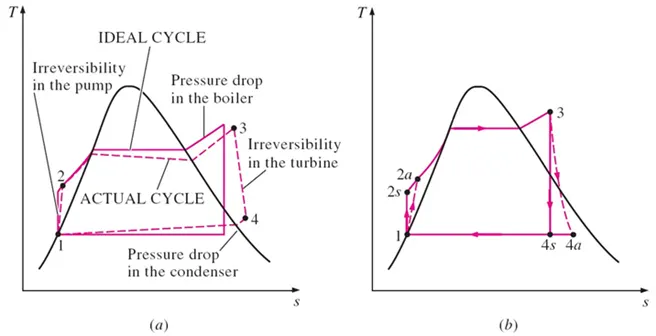
Based on the variation the thermal efficiency of pump and turbine changes. The below are formulas.

INCREASE THE EFFICIENCY OF THE RANKINE CYCLE: the following are methods to enhance efficiency. The basic idea behind all the modifications to increase the thermal efficiency of a power cycle is the same: Increase the average temperature at which heat is transferred to the working fluid in the boiler, or decrease the average temperature at which heat is rejected from the working fluid in the condenser.
Lowering the Condenser Pressure (Lowers T_low, avg): To take advantage of the increased efficiencies at low pressures, the condensers of steam power plants usually operate well below the atmospheric pressure. There is a lower limit to this pressure depending on the temperature of the cooling medium.
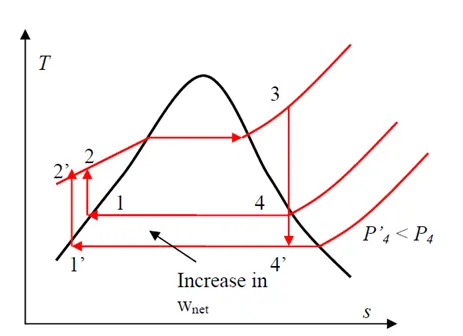
Side effect: Lowering the condenser pressure increases the moisture content of the steam at the final stages of the turbine.
Superheating the Steam to High Temperatures (Increases Thigh,avg)
Both the net work and heat input increase as a result of superheating the steam to a higher temperature. The overall effect is an increase in thermal efficiency since the average temperature at which heat is added increases. Superheating to higher temperatures decreases the moisture content of the steam at the turbine exit, which is desirable. The temperature is limited by metallurgical considerations. Presently the highest steam temperature allowed at the turbine inlet is about 620°C.
Increasing the Boiler Pressure
For a fixed turbine inlet temperature, the cycle shifts to the left and the moisture content of steam at the turbine exit increases. This side effect can be corrected by reheating the steam. Increasing the operating pressure of the boiler leads to an increase in the temperature at which heat is transferred to the steam and thus raises the efficiency of the cycle. The below is the picture depicts.
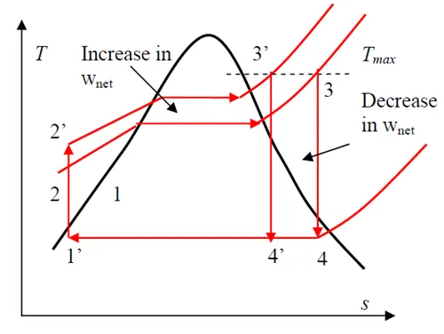
Note that for a fixed turbine inlet temperature, the cycle shifts to the left and the moisture content of the steam at the turbine exit increases. This undesirable side effect can be corrected by reheating the steam.
The Ideal Reheat Rankine Cycle
To take advantage of the increased efficiencies at higher boiler pressure without facing the excessive moisture at the final stages of the turbine, reheating is used. In the ideal reheating cycle, the expansion process takes place in two stages, that is the high-pressure and low-pressure turbines.
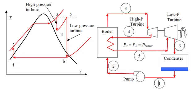
The total heat input and total turbine work output for a reheat cycle become:

The incorporation of the single reheat in a modern power plant improves the cycle efficiency by 4 to 5 percent by increasing the average temperature at which heat is transferred to the steam.
The Ideal Regenerative Rankine Cycle
The regeneration process in steam power plants is accomplished by extracting (or bleeding) steam from turbine at various stages and feed that steam in heat exchanger where the feedwater is heated. These heat exchangers are called regenerator or feedwater heater (FWH). FWH also help removing the air that leaks in at the condenser (de-aerating the feedwater). There are two types of FWH’s, open and closed.
Open (Direct‐Contact) Feedwater Heaters
An open FWH is basically a mixing chamber where the steam extracted from the turbine mixes with the feedwater exiting the pump. Ideally, the mixture leaves the heater as a saturated liquid at the heater pressure. The following are the features of the OFWH:
- Simple
- inexpensive
- good heat transfer characteristics
- bring feedwater to the saturation state
- a pump is required for each FWH
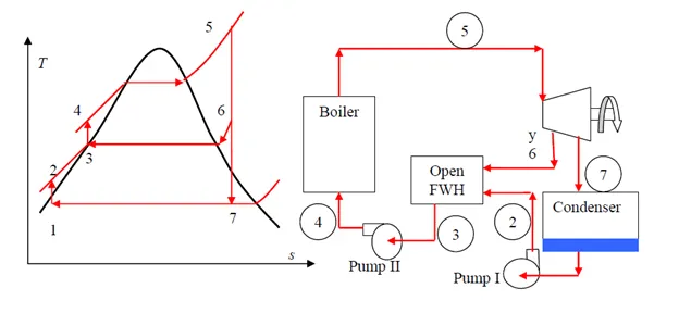
Based on above figure, the heat and work interactions of a regenerative Rankine cycle with one FWH can be expressed per unit mass of steam flowing through the boiler as:
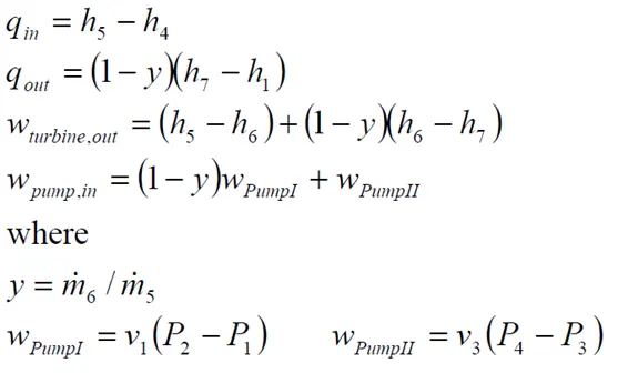
Thermal efficiency of the Rankine cycle increases as a result of regeneration since FWH raises the average temperature of the water before it enters the boiler. Many large power plants have as many as 8 FWH’s.
Closed Feedwater Heaters
In closed FWH, heat is transferred from the extracted steam to the feedwater without any mixing taking place. Thus; two streams can be at different pressures, since they don’t mix. In an ideal closed FWH, the feedwater is heated to the exit temperature of the extracted steam, which ideally leaves the heater as a saturated liquid at the extraction pressure. The below T-S diagram depicts it.
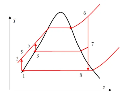
The below is the picture that depicts Ideal regenerative Rankine cycle with a closed FWH.
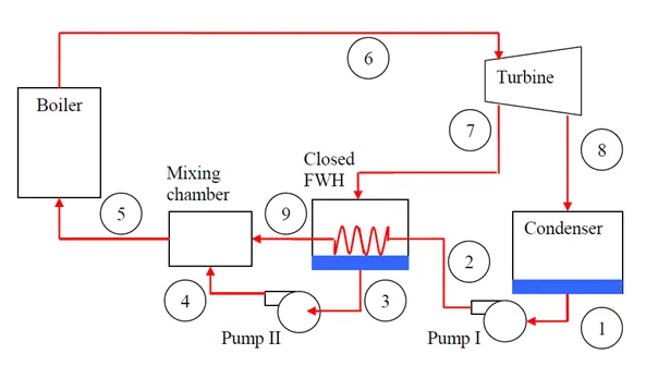
The following features of Closed FWH:
- More complex (internal tubing)
- less effective (no mixing)
- do not require a pump for each FWH
The "dryness fraction", x, gives the fraction by mass of gaseous water in the wet region, the remainder being droplets of liquid.
The ratio of the compressor work to the turbine work is called the back-work ratio. Sometimes, more than one-half of the turbine work may be used by the compressor.
MATLAB CODE FOR RANKINE CYCLE SIMULATOR STEP-BY-STEP DESCRIPTION
Usually, it is good practice to begin the program with clearing all the previous inputs/ data, closing all the previous plots/figures, and clearing command windows. Hence use below code to do that.
%% RANKINE CYCLE SIMULATOR
clear all                               % Clear all the previous inputs and data
close all                               % Close all plots and figure
clc                                     % Clear the command windows
First start with 'fprintf' command to print the name of the simulator in command window. To skip next line or to leave next line blank use ‘n’ as ‘enter’ button on the keyboard.
Secondly define all the process sequences so that user can understand the sequence of the Rankine cycle processes. Again use skip for proper organized presentation.
%% Print Simulator name
fprintf('               RANKINE CYCLE SIMULATOR            n');

fprintf('n') % skip line bank

%% Define/ print all the process in command box
disp('1-2 is Isentropic expansion in Turbine');
disp('2-3 is Constant pressure heat removal in the Condenser');
disp('3-4 is Isentropic compression in the Pump');
disp('4-1 is Constant Pressure heat addition in the Boiler');

fprintf('n') % skip line bank
After that provide entities for the user which ask for the inputs as per following code:-
%% Entity requre to set input parameters
p1 = input('Enter of pressure at turbine inlet, p1(bar)     = ');
T1 = input('Enter of temperature at turbine inlet, T1(°C)   = ');
p2 = input('Enter of temperature at condenser inlet, p2(bar)= ');

fprintf('n')
Now, program the code to calculate entities at each point of the Rankine cycle. In normal practice we use Steam Table to find out the respective values but in this case we are going to use XSteam function to extract the value of properties in relation of other entities.
To select proper steam or liquid condition we refer T-S chart which we understood before.
For Example at point 1
Steam is at superheated reason according to T-S chart so we select ‘h_pT Entalpy as a function of pressure and temperature’ as it is not on saturated line and we have the input value of pressure and temperature at inlet on the turbine, using that we can find out value for enthalpy ‘h1’at point 1.
By using same procedure now we can find out value for Entropy ‘s1’.
So, we got value of entities for T-S and H-S plot at inlet of turbine, at point 1.
%% Extracting data - defining variables
%% [1] Property of steam at point 1
     % Steam at the entry of the turbine
h1 = XSteam('h_pT', p1, T1);
s1 = XSteam('s_pT', p1, T1);
Lets jump toward point 2, which is exit of turbine and also entry point of condenser
As it 1-2 was Isentropic expansion of steam in Turbine entropy will be same so s1= s2
Now their will be chances the vapors can leave the turbine could be superheated in some cases so we have to define it for both condition for that we are going to use both case using ‘if’,’else’ conditions. Using the relation of the dryness fraction we are going to implement that condition
Dryness fraction 'x">x' can be calculated by following way,
`S2=(Sf2)+x*(Sfg2)`
`Sfg2=Sg2-Sf2`
:. `X2=(S2-Sf2)/(Sfg2)`
Then, temperature at point 2 can be calculated using following way
`S2=Sg2+(CpV2)*log((T2)/(Ts2))`
where,
CpVp">CpV2= Saturated vapour heat capacity
`log((T2)/(Ts2))=(S2-Sg2)/(CpV2)`
:. `(T2)/(Ts2)=exp((S2-Sg2)/(CpV2))`
:. `T2=Ts2*exp((S2-Sg2)/(CpV2))`
Next, to calculate enthalpy use below formulas
hear to calculate enthalpy we are going to use condition. if condition of steam is vapour +liquid then we use below formula:-
`h2=hf2+x2*hfg2`
Else, steam will be at its superheated condition so we implemet following formula for that:-
`h2=hg2+CpV2*(T2-Ts2)`
So, the coding at point 2 will be-
%% [2] Property of steam at point 2
     % Steam at the exit of the turbine

s2 = s1;
%For Dryness factor s2 = sf2 + x(sfg)
sf2 = XSteam('sL_p',p2);
sg2 = XSteam('sV_p',p2);
sfg2 = sg2-sf2;

if(s2<=sg2)
    x2 = (s2-sf2)/(sfg2);
else
    x2 = 1;
end

Ts2 = XSteam('Tsat_p',p2);

if (x2<1)
    T2 = Ts2;
else
    % s2 = sg2+CpV2*(log(T2/Ts2))
    % CpV_p Saturated vapour heat capacity
    CpV2 = XSteam('CpV_p',p2);
    %(log(T2/Ts2)) = (s2-sg2)/CpV2
    % T2/Ts2 = exp((s2-sg2)/CpV2)
    % T2 = Ts2 * exp((s2-sg2)/CpV2)
    % add 273.15 to convert tempreture unit from degree Celsius to Kelvin
    T_2 = (Ts2+273.15)*exp((s2-sg2)/CpV2);
    T2 = T_2-273.15;
end

x2 = (s2-sf2)/(sfg2);
hf2 = XSteam('hL_p',p2);
hg2 = XSteam('hV_p',p2);
hfg2 = hg2-hf2;
%h2 = XSteam('h_ps',p2,s2);
if (x2<1)
    h2 = hf2 + x2*hfg2;
else
    h2 = hg2 + CpV2*(T2-Ts2);
end
Point 3 will be always positioned on the liquid saturated line as phase change occur in the condenser at constant pressure. From 2-3 heat is rejected at constant pressure in which vapor give its latent heat and convert into liquid water.
Other entities, Enthalpy, entropy, and Temperature, can be calculated using steam table or XSteam function, considering they are on the saturated liquid line.
%% [3] Property of steam at point 3
     % water and vapors after leaving condenser
p3 = p2;
h3 = hf2;
s3 = sf2;
T3 = Ts2;
After condensation, water is pumped with water pump towards the boiler. Pump pressurize the water from p3 to p1 so p1 is equal to p4.
This is Isentropic compression process where entropy remain same.
Here we consider reheating of water in order to improve net work, which increase the temperature and entropy of the system
In this process enthalpy also increases.
To calculate Enthalpy
Work Done by Pump:-
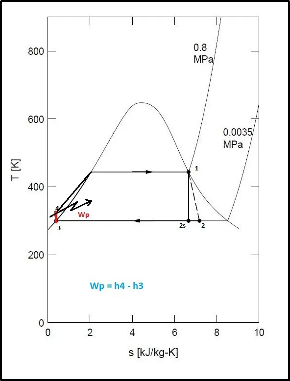
Energy in working fluid at output deducted by energy at input. Basicaly enthalpy difference.
`Wp=h4-h3`
and `Wp=v3(P4-p3)`
find `v3` from XSteam function.
:. `Wp=v3(P4-p3)*100`
:. `h4=h3+Wp`
To calculate temperature
`S4=Sf4-CpL4*log((Ts4)/(T4))`
find out the values for sf4">sf4, Ts4">Ts4 and CpL4">CpL4 From XSteam function.
:. `(Ts4)/(T4)=exp((Sf4-S4)/(CpL4))`
:. `T4=(Ts4)/exp((Sf4-S4)/(CpL4))`
OR
`T4=(T3)/((P3)/(P4))^((K-1)/K)`
where,
`K=(Cp4)/(Cv4)`
value of `Cp4` and `Cv4` find with the help of XSteam function.
After implementing above formulas codes will look line this :-
%% [4] Property of steam at point 4
     % Water after leaving pump
p4 = p1;
s4 = s3;
%h4 = XSteam('h_ps',p4,s4);
%T4 = XSteam('T_ps',p4,s4);
% Work done to run pump = v3(p4-p3) = h4-h3
v3 = XSteam('vL_p',p3);
Wp = v3*(p4-p3)*100;
h4 = h3 + Wp;


% s4 = sf4-cpL4*log(Ts4/T4)
sf4 = XSteam('sL_p',p4);
Ts4 = XSteam('Tsat_p',p4);
CpL4 = XSteam('CpL_p',p4);
% log(Ts4/T4)=(sf4-s4)/CpL4
% Ts4/T4 = exp((sf4-s4)/CpL4)
T4 = Ts4/(exp((sf4-s4)/CpL4));


%----------- OR -----------%
%Cp4 = XSteam('Cp_ps',p4,s4);
%Cv4 = XSteam('Cv_ps',p4,s4);
%k = Cp4/Cv4;
%T4 = T3/(p3/p4)^((k-1)/k);
Upto this point, we got our state points for vapor and water, by using all the enthalpy at this points we can calculate Work done by each component in the system as Enthalpy differences indicate amount of energy produce or consumed by component.
Work done by Turbine:-
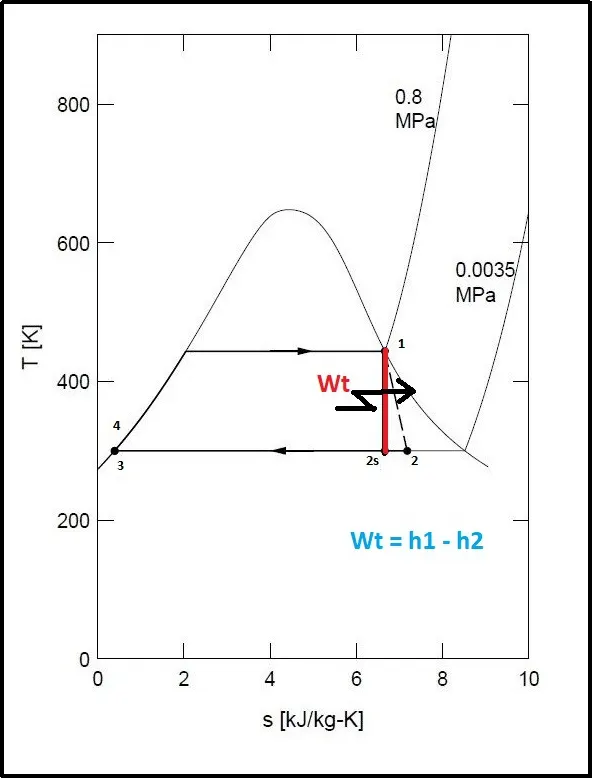
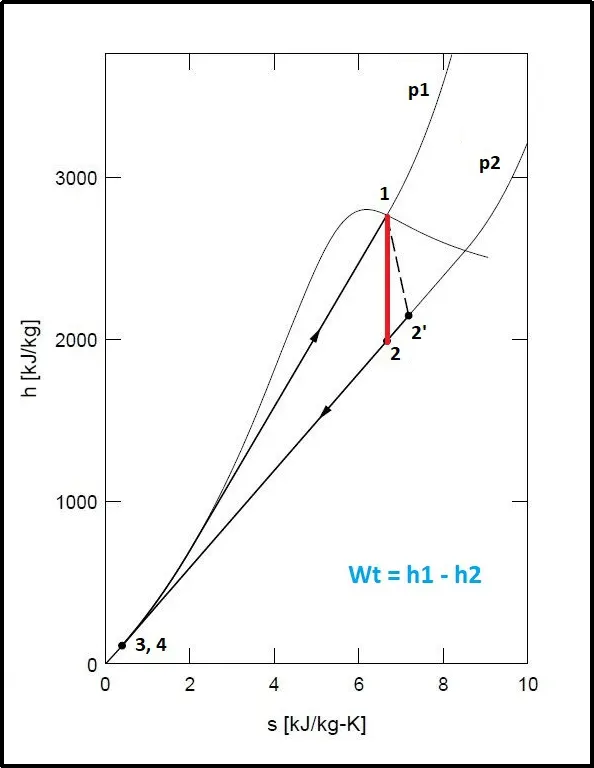
Work output from turbine can be calculated by deducting energy produce from energy supply.
`Wt=h1-h2`
%% Work done by Turbine
Wt = h1 - h2;
Net work :-
Net work is work supplied removed from total work generated in the system.
`Wnet = Wt-Wp`
%% Net work
Wnet = Wt - Wp;
Back work Ratio:-
Back work Ratio (BWR) is the ratio of pump work to turbine work.
`BWR=(Wp)/(Wt)`
%% Back work Ratio
BWR = (Wp/Wt);
Heat into the system:-
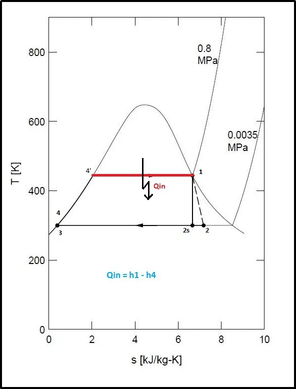
It is the total heat supplied in boiler, calculated by enthalpy difference at boiler in and out.
`Q Input = h1-h4`
%% Heat into the system
Qin = h1 - h4;
Heat Out of the system:-
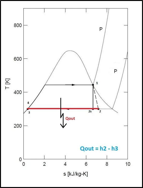
It is the total heat Rejected in condenser, calculated by enthalpy difference at condenser in and out.
`Qoutput = h2-h3`
%% Heat Out of the system
Qout = h2 - h3;
Thermal Efficiency:-
The thermal efficiency of the Rankine cycle is the ratio between the work produced by the steam turbine that has been reduced by the pump work, with the incoming heat energy from the boiler.
`Teff = (1-(Qout)/(QInput))*100`
%% Thermal Efficiency
eff = (1-(Qout/Qin))*100;
Specific Steam Consumption:-
Specific Steam consumption is the ratio of mass flow rate to the power .
It relates the power output to the steam flow necessary to produce steam. The steam flow indicates the size of plart, and the specific steam consumption is a means whereby the relative sizes of different plants can be compared.
The specific steam consumption is the steam flow in kw/h required to develop 1 kw power.
`SSC= (mass flow rate)/(power)`
%% Specific Steam Consumption
   % SSC = mass flow rate/power
SSC = (3600/Wnet);
Find out all the required point on the saturated vapour and liquid line, from XSteam function.
%% Calculating temperature, entropy and enthalpy at the saturated vapour and liquid line
   % Line for Plotting
T1_1 = XSteam('Tsat_p',p1);
T4_1 = T1_1;
s4_1 = XSteam('sL_p',p4);
hf4  = XSteam('hL_p',p4);
h4_1  = hf4;
s1_1 = XSteam('sV_p',p1);
h1_1 = XSteam('hV_p',p1);
T2_1 = XSteam('T_ps',p2,s2);
Extract out all the entopy, enthalpy points at approx 0 bar pressure from XSteam function to plot saturated liquid - vapour line.
%% Create Entophy Enthapy point at 0 constant pressure range
p = 0.01:0.01:400;
for i = 1:length(p)
    T(i) = XSteam('Tsat_p',p(i));
    sf(i) = XSteam('sL_T',p(i));
    sg(i) = XSteam('sv_T',p(i));
    hf(i) = XSteam('hl_T',p(i));
    hg(i) = XSteam('hv_T',p(i));
end
Plotting T-S diagram:-
First plot saturated liquid - vapour line
Then plot other entities using calculated point. use range of data to create proper curve.
%% Plotting T-S diagram
figure(1)
hold on

% Plot saturated vapour and liquid line
plot(sf,p,':','color','g','linewidth',2)
plot(sg,p,':','color','g','linewidth',2)

% [1-2] Isentropic expansion of steam in Turbine
plot([s1 s2],[T1 T2], 'm', 'linewidth',1)


% [2-3] Constant pressure heat removal in the Condenser
if (x2<1)
    str2=0;
    plot(s2,T2,'.');
    plot([s2 s3],[T2 T3],'k', 'linewidth',1);
else
    st2 = linspace(s2,sg2,500);
    for j = 1:length(st2)
        Tt2(j) = XSteam('T_ps',p2,st2(j));
    end
    plot(st2,Tt2,'m', 'linewidth',1);
    plot([sg2 s3],[T3 T3],'m', 'linewidth',1);
end


% [3-4] Isentropic compression of water in the Pump
plot([s3 s4],[T3 T4], 'b', 'linewidth',1)

Tr = linspace(T4,T1_1,20);
hr = linspace(h4,hf4,20);
for r = 1:length(hr)
    sr(r) = XSteam('s_ph',p4,hr(r));
end
plot(sr,Tr,'b','linewidth',1)

sp1 = linspace(s4,s4_1,500);
for f = 1:length(sp1)
    Tp1(f) = XSteam('T_ps',p1,sp1(f));
end
plot(sp1,Tp1,'color','c','linewidth',2)


% [4-1] Constant Pressure heat addition in the Boiler
plot([s4_1 s1_1],[T4_1 T1_1], 'r', 'linewidth',1)
sb1 = linspace(s1_1,s1,500);
for l = 1:length(sb1)
    Tc1(l) = XSteam('T_ps',p1,sb1(l));
end
plot(sb1, Tc1, 'r', 'linewidth',1)


% [1-2-3-4] Labeling points
text(s1+0.1,T1,'1')
text(s1_1-0.3,T1_1-10,"1'")
text(s2+0.1,T2,'2')
if (x2<1)
   str2=0;
else
   text(sg2+0.1,T3,"2'")
end
text(s3,T3-20,'3')
text(s4,T4+20,'4')
text(s4_1,T4_1-10,"4'")

title('Temperature vs Entropy plot')            % Title for the diagram
xlabel('S (Entropy in J/K)')                    % label X-axis
ylabel('T (Temperature in °C)')                 % label Y-axis

% Legend for saturated line
legend('saturated liquid and vapour line','location','northwest')
grid on                                         % Turn on the grid
hold off                                        % Turn off hold on of current plot
Output of Plot T-S diagram:-
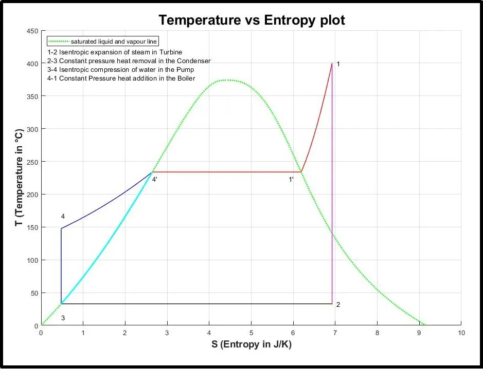
Plotting h-s diagram:-
First plot saturated liquid - vapour line
Then plot other entities using calculated point. use range fo data to create proper curve.
following are the codes to plot h-s diagram
%% Plotting h-s diagram
figure(2)
hold on

% Plot saturated vapour and liquid line
plot(sf, hf,':','color','g','linewidth',2)
plot(sg, hg,':','color','g','linewidth',2)

% [1-2] Isentropic expansion of steam in Turbine
plot([s1 s2],[h1 h2],'m','linewidth',1)

% [2-3] Constant pressure heat removal in the Condenser
plot([s2 s3],[h2 h3],'k','linewidth',1)

% [3-4] Isentropic compression of water in the Pump
plot([s3 s4],[h3 h4],'b','linewidth',1)

% [4-1] Constant Pressure heat addition in the Boiler
hc = linspace(h4,h4_1,100);
for k = 1:length(hc);
    sch(k) = XSteam('s_ph',p1,hc(k));
end
plot(sch,hc,'r','linewidth',1)
plot([s4_1 s1],[h4_1 h1],'r','linewidth',1)


% [1-2-3-4] Labeling points
text(s1+0.1,h1,'1')
text(s2+0.1,h2,'2')
text(s3+0.3, h3,'3,4')
text(s4+0.3, h4,'3,4')

title('Enthalpy vs Entropy plot')               % Title for the diagram
xlabel('S (Entropy in KJ/kgk)')                 % label X-axis
ylabel('H (Enthalpy in KJ/kg)')                 % label Y-axis

% Legend for saturated line
legend('saturated liquid and vapour line','location','northwest')
grid on                                         % Turn on the grid
hold off                                        % Turn off hold on of current plot
Output of above code to create h-s diagram:-
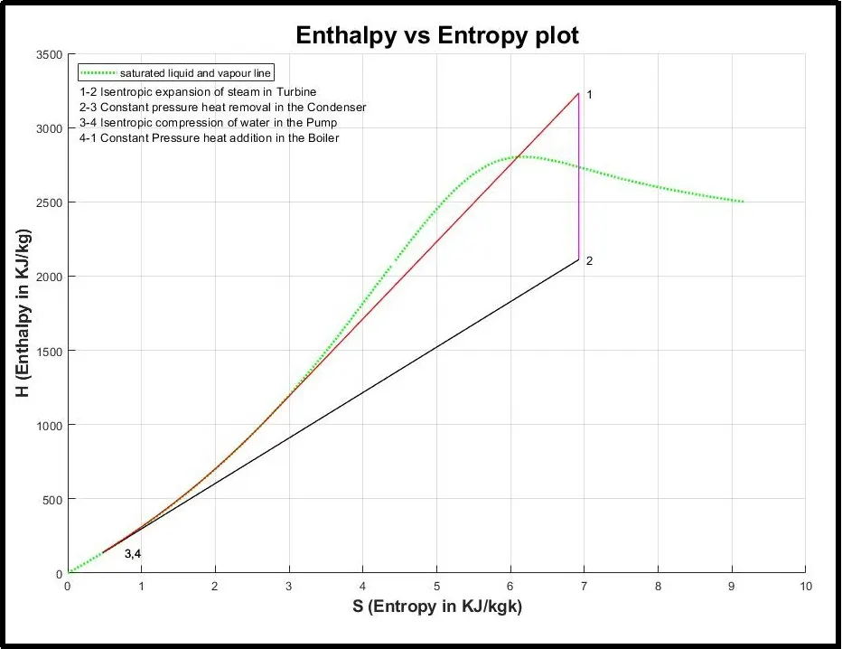
Print all the results in the command window:-
following are the codes to print all the Results and output of the Rankine Cycle Simulator
%% Displaying Results
   % print all the state points parameters and outputs in command window
fprintf('     Results    n')

fprintf('n') % skip line bank


fprintf('At State Point 1 n')
fprintf('p1: %.3f bar n',p1)
fprintf('T1: %.3f °C n', T1)
fprintf('h1: %.3f KJ/Kg n',h1)
fprintf('s1: %.3f Kj/Kgk n',s1)

fprintf('n') % skip line bank


fprintf('At State Point 2 n')
fprintf('p2: %.3f bar n',p2)
fprintf('T2: %.3f °C n', T2)
fprintf('h2: %.3f KJ/Kg n',h2)
fprintf('s2: %.3f Kj/Kgk n',s2)

fprintf('n') % skip line bank


fprintf('At State Point 3 n')
fprintf('p3: %.3f bar n',p3)
fprintf('T3: %.3f °C n', T3)
fprintf('h3: %.3f KJ/Kg n',h3)
fprintf('s3: %.3f Kj/Kgk n',s3)

fprintf('n') % skip line bank


fprintf('At State Point 4 n')
fprintf('p4 : %.3f bar n',p4)
fprintf('T4 : %.3f °C n', T4)
fprintf('h4 : %.3f KJ/Kg n',h4)
fprintf('s4 : %.3f Kj/Kgk n',s4)
Results:-
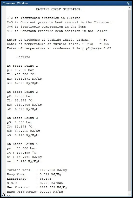
Complete Matlab Program for Rankine cycle Simulator
%% RANKINE CYCLE SIMULATOR
clear all                               % Clear all the previous inputs and data
close all                               % Close all plots and figure
clc                                     % Clear the command windows

%% Print Simulator name
fprintf('               RANKINE CYCLE SIMULATOR            n');

fprintf('n') % skip line bank

%% Define/ print all the process in command box
disp('1-2 is Isentropic expansion in Turbine');
disp('2-3 is Constant pressure heat removal in the Condenser');
disp('3-4 is Isentropic compression in the Pump');
disp('4-1 is Constant Pressure heat addition in the Boiler');

fprintf('n') % skip line bank

%% Entity required to set input parameters
%Turbine inlet temperature = 400 °C
%Turbine inlet pressure = 30 bars
%Turbine outlet pressure = 0.05 bars = Condenser inlet pressure
p1 = input('Enter  pressure at turbine inlet, p1(bar)  = ');
T1 = input('Enter  temperature at turbine inlet, T1(°C) = ');
p2 = input('Enter  pressure at turbine outlet, p2(bar) = ');

fprintf('n')

%% Extracting data - defining variables

%% [1] Property of steam at point 1
     % Steam at the entry of the turbine
h1 = XSteam('h_pT', p1, T1);
s1 = XSteam('s_pT', p1, T1);

%% [2] Property of steam at point 2
     % Steam at the exit of the turbine

s2 = s1;
%For Dryness factor s2 = sf2 + x(sfg)
sf2 = XSteam('sL_p',p2);
sg2 = XSteam('sV_p',p2);
sfg2 = sg2-sf2;

if(s2<=sg2)
    x2 = (s2-sf2)/(sfg2);
else
    x2 = 1;
end

Ts2 = XSteam('Tsat_p',p2);

if (x2<1)
    T2 = Ts2;
else
    % s2 = sg2+CpV2*(log(T2/Ts2))
    % CpV_p Saturated vapour heat capacity
    CpV2 = XSteam('CpV_p',p2);
    %(log(T2/Ts2)) = (s2-sg2)/CpV2
    % T2/Ts2 = exp((s2-sg2)/CpV2)
    % T2 = Ts2 * exp((s2-sg2)/CpV2)
    % add 273.15 to convert tempreture unit from degree Celsius to Kelvin
    T_2 = (Ts2+273.15)*exp((s2-sg2)/CpV2);
    T2 = T_2-273.15;
end

x2 = (s2-sf2)/(sfg2);
hf2 = XSteam('hL_p',p2);
hg2 = XSteam('hV_p',p2);
hfg2 = hg2-hf2;
%h2 = XSteam('h_ps',p2,s2);
if (x2<1)
    h2 = hf2 + x2*hfg2;
else
    h2 = hg2 + CpV2*(T2-Ts2);
end

%% [3] Property of steam at point 3
     % water and vapors after leaving condenser
p3 = p2;
h3 = hf2;
s3 = sf2;
T3 = Ts2;

%% [4] Property of steam at point 4
     % Water after leaving pump
p4 = p1;
s4 = s3;
%h4 = XSteam('h_ps',p4,s4);
%T4 = XSteam('T_ps',p4,s4);
% Work done to run pump = v3(p4-p3) = h4-h3
v3 = XSteam('vL_p',p3);
Wp = v3*(p4-p3)*100;
h4 = h3 + Wp;


% s4 = sf4-cpL4*log(Ts4/T4)
sf4 = XSteam('sL_p',p4);
Ts4 = XSteam('Tsat_p',p4);
CpL4 = XSteam('CpL_p',p4);
% log(Ts4/T4)=(sf4-s4)/CpL4
% Ts4/T4 = exp((sf4-s4)/CpL4)
T4 = Ts4/(exp((sf4-s4)/CpL4));


%----------- OR -----------%
%Cp4 = XSteam('Cp_ps',p4,s4);
%Cv4 = XSteam('Cv_ps',p4,s4);
%k = Cp4/Cv4;
%T4 = T3/(p3/p4)^((k-1)/k);

%% Work done by Turbine
Wt = h1 - h2;

%% Net work
Wnet = Wt - Wp;

%% Back work Ratio
BWR = (Wp/Wt);

%% Heat into the system
Qin = h1 - h4;

%% Heat Out of the system
Qout = h2 - h3;

%% Thermal Efficiency
eff = (1-(Qout/Qin))*100;

%% Specific Steam Consumption
   % SSC = mass flow rate/power
SSC = (3600/Wnet);

%% Calculating temperature, entropy and enthalpy at the saturated vapour and liquid line
   % Line for Plotting
T1_1 = XSteam('Tsat_p',p1);
T4_1 = T1_1;
s4_1 = XSteam('sL_p',p4);
hf4  = XSteam('hL_p',p4);
h4_1  = hf4;
s1_1 = XSteam('sV_p',p1);
h1_1 = XSteam('hV_p',p1);
T2_1 = XSteam('T_ps',p2,s2);

%% Create Entophy Enthapy point at 0 constant pressure range
p = 0.01:0.01:400;
for i = 1:length(p)
    T(i) = XSteam('Tsat_p',p(i));
    sf(i) = XSteam('sL_T',p(i));
    sg(i) = XSteam('sv_T',p(i));
    hf(i) = XSteam('hl_T',p(i));
    hg(i) = XSteam('hv_T',p(i));
end


%% Plotting T-S diagram
figure(1)
hold on

% Plot saturated vapour and liquid line
plot(sf,p,':','color','g','linewidth',2)
plot(sg,p,':','color','g','linewidth',2)

% [1-2] Isentropic expansion of steam in Turbine
plot([s1 s2],[T1 T2], 'm', 'linewidth',1)


% [2-3] Constant pressure heat removal in the Condenser
if (x2<1)
    str2=0;
    plot(s2,T2,'.');
    plot([s2 s3],[T2 T3],'k', 'linewidth',1);
else
    st2 = linspace(s2,sg2,500);
    for j = 1:length(st2)
        Tt2(j) = XSteam('T_ps',p2,st2(j));
    end
    plot(st2,Tt2,'m', 'linewidth',1);
    plot([sg2 s3],[T3 T3],'m', 'linewidth',1);
end


% [3-4] Isentropic compression of water in the Pump
plot([s3 s4],[T3 T4], 'b', 'linewidth',1)

Tr = linspace(T4,T1_1,20);
hr = linspace(h4,hf4,20);
for r = 1:length(hr)
    sr(r) = XSteam('s_ph',p4,hr(r));
end
plot(sr,Tr,'b','linewidth',1)

sp1 = linspace(s4,s4_1,500);
for f = 1:length(sp1)
    Tp1(f) = XSteam('T_ps',p1,sp1(f));
end
plot(sp1,Tp1,'color','c','linewidth',2)


% [4-1] Constant Pressure heat addition in the Boiler
plot([s4_1 s1_1],[T4_1 T1_1], 'r', 'linewidth',1)
sb1 = linspace(s1_1,s1,500);
for l = 1:length(sb1)
    Tc1(l) = XSteam('T_ps',p1,sb1(l));
end
plot(sb1, Tc1, 'r', 'linewidth',1)


% [1-2-3-4] Labeling points
text(s1+0.1,T1,'1')
text(s1_1-0.3,T1_1-10,"1'")
text(s2+0.1,T2,'2')
if (x2<1)
   str2=0;
else
   text(sg2+0.1,T3,"2'")
end
text(s3,T3-20,'3')
text(s4,T4+20,'4')
text(s4_1,T4_1-10,"4'")

title('Temperature vs Entropy plot')            % Title for the diagram
xlabel('S (Entropy in J/K)')                    % label X-axis
ylabel('T (Temperature in °C)')                 % label Y-axis

% Legend for saturated line
legend('saturated liquid and vapour line','location','northwest')

grid on                                         % Turn on the grid
hold off                                        % Turn off hold on of current plot


%% Plotting h-s diagram
figure(2)
hold on

% Plot saturated vapour and liquid line
plot(sf, hf,':','color','g','linewidth',2)
plot(sg, hg,':','color','g','linewidth',2)

% [1-2] Isentropic expansion of steam in Turbine
plot([s1 s2],[h1 h2],'m','linewidth',1)

% [2-3] Constant pressure heat removal in the Condenser
plot([s2 s3],[h2 h3],'k','linewidth',1)

% [3-4] Isentropic compression of water in the Pump
plot([s3 s4],[h3 h4],'b','linewidth',1)

% [4-1] Constant Pressure heat addition in the Boiler
hc = linspace(h4,h4_1,100);
for k = 1:length(hc);
    sch(k) = XSteam('s_ph',p1,hc(k));
end
plot(sch,hc,'r','linewidth',1)
plot([s4_1 s1],[h4_1 h1],'r','linewidth',1)


% [1-2-3-4] Labeling points
text(s1+0.1,h1,'1')
text(s2+0.1,h2,'2')
text(s3+0.3, h3,'3,4')
text(s4+0.3, h4,'3,4')

title('Enthalpy vs Entropy plot')               % Title for the diagram
xlabel('S (Entropy in KJ/kgk)')                 % label X-axis
ylabel('H (Enthalpy in KJ/kg)')                 % label Y-axis

% Legend for saturated line
legend('saturated liquid and vapour line','location','northwest')
grid on                                         % Turn on the grid
hold off                                        % Turn off hold on of current plot

%% Displaying Results
   % print all the state points parameters and outputs in command window
fprintf('     Results    n')

fprintf('n') % skip line bank


fprintf('At State Point 1 n')
fprintf('p1: %.3f bar n',p1)
fprintf('T1: %.3f °C n', T1)
fprintf('h1: %.3f KJ/Kg n',h1)
fprintf('s1: %.3f Kj/Kgk n',s1)

fprintf('n') % skip line bank


fprintf('At State Point 2 n')
fprintf('p2: %.3f bar n',p2)
fprintf('T2: %.3f °C n', T2)
fprintf('h2: %.3f KJ/Kg n',h2)
fprintf('s2: %.3f Kj/Kgk n',s2)

fprintf('n') % skip line bank


fprintf('At State Point 3 n')
fprintf('p3: %.3f bar n',p3)
fprintf('T3: %.3f °C n', T3)
fprintf('h3: %.3f KJ/Kg n',h3)
fprintf('s3: %.3f Kj/Kgk n',s3)

fprintf('n') % skip line bank


fprintf('At State Point 4 n')
fprintf('p4 : %.3f bar n',p4)
fprintf('T4 : %.3f °C n', T4)
fprintf('h4 : %.3f KJ/Kg n',h4)
fprintf('s4 : %.3f Kj/Kgk n',s4)

fprintf('n') % skip line bank


fprintf('Turbine Work   : %.3f KJ/Kg  n',Wt)
fprintf('Punp Work      : %.3f KJ/Kg  n',Wp)
fprintf('Efficiency     : %.2f%%',eff)
fprintf('n')
fprintf('S.S.C          : %.3f KJ/KWh n',SSC)
fprintf('Net Work out   : %.3f KJ/Kg  n',Wnet)
fprintf('Back work Ratio: %.4f KJ/Kg  n',BWR)

%-----------------------------------end-----------------------------------%