Week 4 - Genetic Algorithm
MATLAB Program to optimize the stalagmite function using Genetic Algorithm and find the global maxima of the function.
Aim
The main aim is to optimize the Stalagmite function using Genetic algorithm and to find the global maxima of the function .
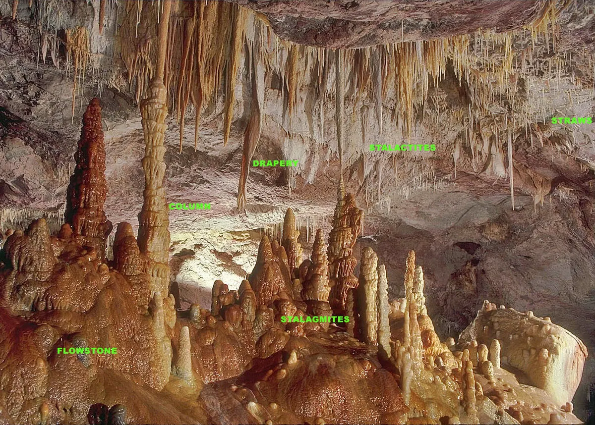
Stalagmites:
A Stalagmite is a type of rock formation that rises from the floor of a cave due to the accumulation of material deposited on the floor from ceiling drippings. Stalagmites are typically composed of calcium carbonate but may consist of lava, mud, peat, pitch, sand, sinter, and amberat (crystallized urine of packrats).
Genetic Algorithm:
In computer science and operations research, a genetic algorithm (GA) is a metaheuristic inspired by the process of natural selection that belongs to the larger class of evolutionary algorithms (EA). Genetic algorithms are commonly used to generate high-quality solutions to optimization and search problems by relying on biologically inspired operators such as mutation, crossover, and selection.
It is inspired by Charles Darwin's theory of natural evolution. This algorithm reflects the process of natural selection where the fittest individuals are selected for reproduction to produce offspring of the next generation.
Charles Darwin’s Theory of Natural Evolution:
The theory of evolution by natural selection, first formulated in Darwin's book "On the Origin of Species" in 1859, is the process by which organisms change over time as a result of changes in heritable physical or behavioral traits. Changes that allow an organism to better adapt to its environment will help it survive and have more offspring.
Evolution by natural selection is one of the best-substantiated theories in the history of science, supported by evidence from a wide variety of scientific disciplines, including paleontology, geology, genetics, and developmental biology.
Working Principle:
Genetic algorithms (GAs) are stochastic search methods based on the principles of natural genetic systems. They perform a search in providing an optimal solution for the evaluation (fitness) function of an optimization problem. GAs deal simultaneously with multiple solutions and use only the fitness function values. While solving an optimization problem using GAs, each solution is coded as a string (called "chromosome") of finite length over a finite alphabet A. Each string or chromosome is considered as an individual. A collection of M (M is finite) such individuals is called a population.
The genetic algorithm starts with a randomly generated population of size M. During the process of iteration, a new population of the same size is generated from the current population using three basic operations on the individuals of the population.
Five phases are considered in a genetic algorithm.
- Initial population
- Fitness function
- Selection
- Crossover
- Mutation
- Initial Population:
- The process begins with a set of individuals which is called a Population. Each individual is a solution to the problem you want to solve.
- An individual is characterized by a set of parameters (variables) known as Genes. Genes are joined into a string to form a Chromosome (solution).
- In a genetic algorithm, the set of genes of an individual is represented using a string, in terms of an alphabet. Usually, binary values are used (string of 1s and 0s). We say that we encode the genes in a chromosome.
- Fitness function:
- The fitness function determines how fit an individual is (the ability of an individual to compete with other individuals). It gives a fitness score to each individual. The probability that an individual will be selected for reproduction is based on its fitness score.
- Selection:
- The idea of the selection phase is to select the fittest individuals and let them pass their genes to the next generation.
- Two pairs of individuals (parents) are selected based on their fitness scores. Individuals with high fitness have more chances to be selected for reproduction.
- Crossover:
- Crossover is the most significant phase in a genetic algorithm. For each pair of parents to be mated, a crossover point is chosen at random from within the genes.
-
For example, consider the crossover point to be 3 as in the figure below:
Offsprings are created by exchanging genes of parents among themselves until the crossover point is reached.
-
The new offspring is then added to the population.
- Mutation:
- In certain new offspring formed, some of their genes can be subjected to a mutation with a low random probability. This implies that some of the bits in the bit string can be flipped.
-
This implies that some of the bits in the bit string can be flipped.
Mutation occurs to maintain diversity within population and prevent premature convergence.
-
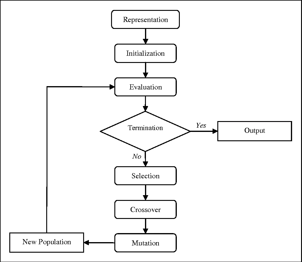
The flowchart for Genetic Algorithm is given below,
Syntax for defining ‘ga’ (Genetic Algorithm) in matlab –
The ‘ga’ syntax in matlab is used to find the minimum of function using genetic algorithm. There are several ways to define the ‘ga’ function depending on the problem being solved. The syntax used for this study is shown below.
- x = ga(fun,nvars)
where,
x = optimal solution/variables;
fun = Objective function;
nvars = Number of variables;
Sometimes ‘[x,fval]’ is used instead of ‘x’ where ‘fval’ gives objective function value at the solution
- x = ga(fun,nvars,A,B,Aeq,Beq,lb,ub)
where,
A, B = Linear inequality constraints
Aeq, Beq = Linear equality constraints
If there are no linear equalities and inequalities, then A, B, Aeq, Beq are set to ‘[ ]’.
- x = ga(fun,nvars,A,B,Aeq,Beq,lb,ub,nonlcon,IntCon,options)
where,
nonlcon = Nonlinear constraints
IntCon = Integer Values
options = Optimization options
If there are no nonlinear constraints and integer values, the nonlcon and IntCon are set to ‘[ ]’.
- Equation for Stalagmite function
The stalagmite function is given as,
`f(x,y)=f1(x)*f2(x)*f1(y)*f2(y)`
where,
`f1(x)=[sin(5.1*pi*x+0.5)]^6`
`f1(y)=[sin(5.1*pi*y+0.5)]^6`
`f2(x)=exp[-4ln(2)*(x-0.0667)^2/0.64]`
`f2(y)=exp[-4ln(2)*(y-0.0667)^2/0.64]`
Genetic algorithm, finds local minima of the finction, but in order to attain the maxima value the ‘-’ sign is placed before the equation.
The Global maxima is as follows
`f(x,y)=-[f1(x)*f2(x)*f1(y)*f2(y)]`
Process of Solving:
The Order in which the code is written is as below
- Write Stalagmite Function.
- Evaluating the stalagmite function.
- Writing the code for Unbounded Inputs.
- Writing the code for the Bounded Inputs.
- Writing the code for the Bounded Inputs with increased population size:
Procedure
- Writing the Stalagmite function:
function [f] = stalagmite(input_vector)

x= input_vector(1);
y= input_vector(2);

f1 = (sin(5.1*pi*x + 0.5)).^6;
f2 = exp(-4*log(2)*((x-0.0667).^2)./0.64);
f3 = (sin(5.1*pi*y + 0.5)).^6;
f4 = exp(-4*log(2)*((y-0.0667).^2)./0.64);

f = -(f1*f2*f3*f4);

end
While using the function at the end as we are using the -ve sign so that the plot will be reversed as we have to find the maxima of the given function using ga.
- Evaluating the stalagmite function:
- The code is written to check if the stalagmite function is returning an output.
- Creates a surface plot showing stalagmite function of input vector.
%% PROVIDING THE SEARCH SPACE FOR THE FUNCTION

    x=linspace(0,0.6,150);
    y=linspace(0,0.6,150);
    [X,Y]=meshgrid(x,y); % Creating a 2D array

    num_cases=50;       %Number of itreation for which the function will evaluate the fitness


%% CREATING THE SURFACE PLOT OF STALAGEMITE FUNCTION

     for i=1:length(X)
         for l=1:length(Y)
             input_vector(1)=X(i,l);
             input_vector(2)=Y(i,l);
             f(i,l)=stalagmite(input_vector);   % calling stalagmite function
         end
     end

surfc(X,Y,-f);       %generating the surfaceplot
shading interp      %To remove the lines produced by the mesh grid

figure(1)
xlabel('x value')
ylabel('y values')
legend('X Values','Y values')
title('Stalagmite Function')
saveas(1, 'Stalagmite.png') % saving plot
RESULT
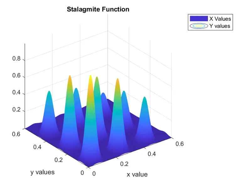
figure below shows the stalagmite function
- Writing the code for Unbounded Inputs:
- In this case we are performing statistical study of genetic algorithm by trying to find optimum value of stalagmite function ( global maxima)
- here we run genetic algorithm without defining any upper and lower limits.
- syntax fpr 'ga' is,
x= ga(fun,nvars)x, to the objective function,fun.nvarsis the dimension (number of design variables) offun.
%% STATISTICAL BEHAVIOUR (UNBOUNDED)/Random samples

tic                             %calculating the study time through tic and toc command
for i=1:num_cases

        [inputs,fopt(i)]=ga(@stalagmite,2);    %calculating the optimized value of the function using genetic algoritham
        xopt(i)=inputs(1);                      %at each iteration
        yopt(i)=inputs(2);

end
study1_time=toc                  %displaying the time taken to evaluate

        % PLOTING THE GRAPH
        figure(2)

        subplot(2,1,1) % subplot(m,n,p) divides the current figure into an m-by-n grid and creates axes in the position specified by p
        surfc(X,Y,-f);
        hold on

        shading interp
        plot3(xopt,yopt,-fopt,'marker','o','markersize',5,'markerfacecolor','r');
        xlabel('x values');
        ylabel('y values');
        grid on
        subplot(2,1,2)
        plot(-fopt);
        xlabel('Iterations')
        ylabel('Function Minimum')
        saveas(2,'Unbound Inputs.png')
Result
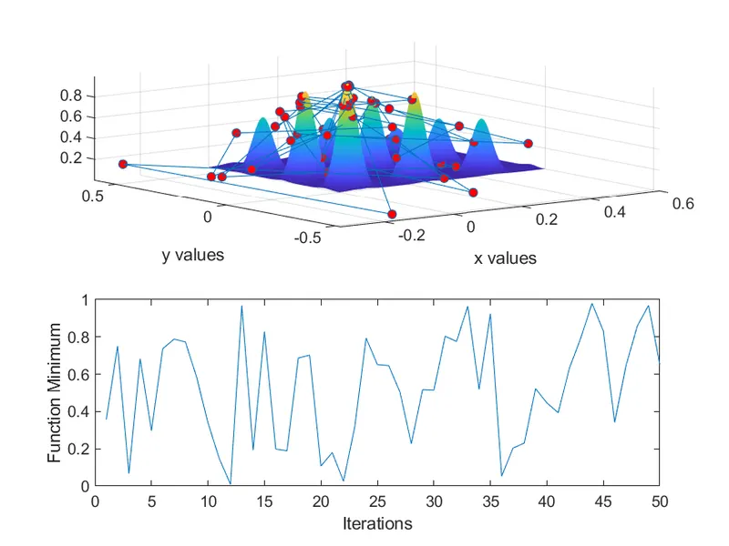
In above plot, it can be observed how the random sampling of the genetic algorithm generates a new optimum value for the function every time the code is run. Although this falls in line with the definition of Genetic Algorithm. Large number of red dots shows that at each iterations 'ga' generates different optimum value for the the stalagmite function.
- Writing the code for the Bounded Inputs:
Here we provide the upper and the lower limit in the 'ga' , so that the search space is reduced with the upper and lower boundary.
%% STATISTICAL BEHAVIOUR (BOUNDED)- sample with upper and lower limits

tic                                %calculating the study time through tic and toc command
 for l=1:num_cases

        [inputs,fopt(l)]=ga(@stalagmite,2,[],[],[],[],[0;0],[0.6;0.6]);   %calculating the optimized value of the functionw ith specified upper and lowe limits
        xopt(l)=inputs(1);
        yopt(l)=inputs(2);

 end
study2_time=toc

    %PLOTTING
figure(3)
subplot(2,1,1)
surfc(x,y,-f)
shading interp
title('Bounded Inputs')
xlabel('x value')
ylabel('y value')

hold on

plot3(xopt,yopt,-fopt, 'marker','o', 'markersize', 5, 'markerfacecolor', 'r')
subplot(2,1,2)
plot(-fopt)
xlabel(' Iterations' )
ylabel('Function Minimum')
saveas(3, 'Bounded Input.png')
Result
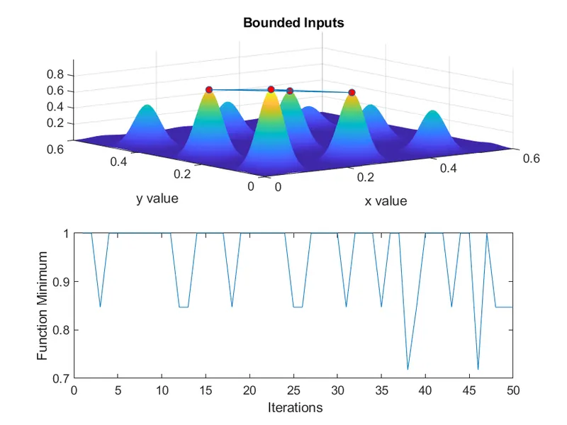
The above results show the convergence of x and y values. The number of red dots are less compared to previous plot.
It is clearly seen from the above that after providing the boundary limits the variation in the optimum value of the function has reduced.
- Writing the code for the Bounded Inputs with modified population size:
- Here in addition of defining upper and lower limits we are increasing population size
- In this study using the ‘optimoptions’ command to increase the size of population.
- The benefit of that will be it will be working on the large set of numbers and which will be led to increase the possibilities of finding the better fitness of the function.
- The drawback is that the time for evaluation will increase.
%% MODIFYING THE NUMBER OF POPULATION ( increasing population size )

 options=optimoptions('ga','populationsize',250)        %increaing the size of population by using
                                                        %optimoptions function

 tic
for l=1:num_cases

    [inputs,fopt(l)]=ga(@stalagmite,2,[],[],[],[],[0;0],[0.6;0.6],[],[],options);
     xopt(l)=inputs(1);
     yopt(l)=inputs(2);

end
study3_time=toc

    %PLOTTING
figure(4)
subplot(2,1,1)
surfc(x,y,-f)
shading interp
title('Bounded Inputs with modified population size')
xlabel('x value')
ylabel('y value')

hold on

plot3(xopt,yopt,-fopt, 'marker','o','markersize',5,'markerfacecolor','r')
subplot(2,1,2)
plot(-fopt)
xlabel('Iterations')
ylabel('Function Minimum')
saveas(4, 'Bounded Inputs with increased population size.png')
Result
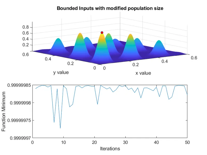
Here, with increased population size and with upper and lower limit values we are getting optimum value (global maxima) of the stalagmite function
Here we can see that there is only one red dot on the stalagmite function and that is the required global maxima point.
Main code for optimizing
% Cleanup
clear
close all
clc

%% PROVIDING THE SEARCH SPACE FOR THE FUNCTION

    x=linspace(0,0.6,150);
    y=linspace(0,0.6,150);
    [X,Y]=meshgrid(x,y); % Creating a 2D array

    num_cases=50;       %Number of itreation for which the function will evaluate the fitness


%% CREATING THE SURFACE PLOT OF STALAGEMITE FUNCTION

     for i=1:length(X)
         for l=1:length(Y)
             input_vector(1)=X(i,l);
             input_vector(2)=Y(i,l);
             f(i,l)=stalagmite(input_vector);   % calling stalagmite function
         end
     end

surfc(X,Y,-f);       %generating the surfaceplot
shading interp      %To remove the lines produced by the mesh grid

figure(1)
xlabel('x value')
ylabel('y values')
legend('X Values','Y values')
title('Stalagmite Function')
saveas(1, 'Stalagmite.png') % saving plot


%% STATISTICAL BEHAVIOUR (UNBOUNDED)/Random samples

tic                             %calculating the study time through tic and toc command
for i=1:num_cases

        [inputs,fopt(i)]=ga(@stalagmite,2);    %calculating the optimized value of the function using genetic algoritham
        xopt(i)=inputs(1);                      %at each iteration
        yopt(i)=inputs(2);

end
study1_time=toc                  %displaying the time taken to evaluate

        % PLOTING THE GRAPH
        figure(2)

        subplot(2,1,1) % subplot(m,n,p) divides the current figure into an m-by-n grid and creates axes in the position specified by p
        surfc(X,Y,-f);
        hold on

        shading interp
        plot3(xopt,yopt,-fopt,'marker','o','markersize',5,'markerfacecolor','r');
        xlabel('x values');
        ylabel('y values');
        grid on
        subplot(2,1,2)
        plot(-fopt);
        xlabel('Iterations')
        ylabel('Function Minimum')
        saveas(2,'Unbound Inputs.png')


%% STATISTICAL BEHAVIOUR (BOUNDED)- sample with upper and lower limits

tic                                %calculating the study time through tic and toc command
 for l=1:num_cases

        [inputs,fopt(l)]=ga(@stalagmite,2,[],[],[],[],[0;0],[0.6;0.6]);   %calculating the optimized value of the functionw ith specified upper and lowe limits
        xopt(l)=inputs(1);
        yopt(l)=inputs(2);

 end
study2_time=toc

    %PLOTTING
figure(3)
subplot(2,1,1)
surfc(x,y,-f)
shading interp
title('Bounded Inputs')
xlabel('x value')
ylabel('y value')

hold on

plot3(xopt,yopt,-fopt, 'marker','o', 'markersize', 5, 'markerfacecolor', 'r')
subplot(2,1,2)
plot(-fopt)
xlabel(' Iterations' )
ylabel('Function Minimum')
saveas(3, 'Bounded Input.png')

%% MODIFYING THE NUMBER OF POPULATION ( increasing population size )

 options=optimoptions('ga','populationsize',250)        %increaing the size of population by using
                                                        %optimoptions function

 tic
for l=1:num_cases

    [inputs,fopt(l)]=ga(@stalagmite,2,[],[],[],[],[0;0],[0.6;0.6],[],[],options);
     xopt(l)=inputs(1);
     yopt(l)=inputs(2);

end
study3_time=toc

    %PLOTTING
figure(4)
subplot(2,1,1)
surfc(x,y,-f)
shading interp
title('Bounded Inputs with modified population size')
xlabel('x value')
ylabel('y value')

hold on

plot3(xopt,yopt,-fopt, 'marker','o','markersize',5,'markerfacecolor','r')
subplot(2,1,2)
plot(-fopt)
xlabel('Iterations')
ylabel('Function Minimum')
saveas(4, 'Bounded Inputs with increased population size.png')

global_maxima = -fopt       % Finding the Global Maxima
Explanation of code
- The code starts with clear all, close all and clc where,
- ‘clear all’ command is used to clear the data stored in the workspace.
- ‘close all’ command is used to close all plots and figures.
- ‘clc’ command is used to clear the command window.
- Then the ‘x’ array and ‘y’ array is defined using ‘linspace’ command to create values at 150 equal intervals.
- A 2D mesh of x and y array is created by using ‘meshgrid’ command and the number of iterations or cases that the code should perform is defined. This is given by n = 50.
- To evaluate the stalagmite function, ‘for’ loop is used where ‘i’ is initialized and for every value of ‘i’ another ‘for’ loop is used to initialize ‘j’.
- The input vector values of ‘xx’ and ‘yy’ are defined and the stalagmite function for these input vector is defined. This will form a basic stalagmite function and we can plot it separately if needed.
- After preparing the inputs needed for the function, next step is to obtain the results for 3 cases of the genetic algorithm. In first case or study, the maximum value of function is found out with no restrictions, no bounds and no limits.
- This is done using ‘for’ loop where we use ‘ga’ syntax to give values for inputs and optimum max value. The stalagmite function is called in ‘ga’ syntax and number of variables ‘nvars’ are 2.
- To know the time that is taken to solve the loop for 50 iterations, ‘tic’ and ‘toc’ command is used before and after the loop respectively.
- Then the function created in the loop is plotted by using ‘surfc’ command for ‘xx, yy and function output’. To neglect the gridlines on the surface and obtain a smooth and clean plot, ‘shading interp’ command is used. The ‘subplot(2,1,1)’ is used to plot multiple plots on same figure which also divides figure in grid of 2x1 and axes to be placed at 1.
- The ‘plot3’ command plots the 3D points at ‘xopt, yopt and optimum value of function’ with ‘o’ shaped and red colour. The labels and title are then provided. Now in the same figure, the values of optimum function ‘fopt’ are plotted for 50 iterations.
- The results of the above case will be different for each time we run the program. To get same value each time, we need to restrict the program within specific bounds namely upper bound and lower bound. The procedure for coding and plottind this procedure is same as Study 1. The only difference is in the ‘ga’ syntax. This time the algorithm is provided lower limits and upper limits as [0;0] and [1;1] respectively.
- After plotting the results for Study 2 or the bounded case, it is observed that the results are not same every time the program terminates. A solution to this problem is to increase the number of cases or iterations.
- So for Study 3, the number of iterations are increased to 300. So for this study, the syntax, “options = optimoptions(‘SolverName’,’Name’,‘Value’)” is used which returns with named parameter ‘Populations’ with the altered values ‘300’.
- The syntax for ‘ga’ contains ‘option’ term and the rest of the code is same as for Study 1 and 2.
- Surfc:
surfc function contours the plot under the surface plot. surfc(X, Y, Z) creates a three-dimensional surface plot with a contour plot underneath. A surface plot is a three-dimensional surface that has solid edge colors and solid face colors. The function plots the values in matrix Z as heights above a grid in the x-y plane defined by X and Y. The color of the surface varies according to the heights specified by Z.
- Shading:
The shading function controls the color shading of surface and patch graphics objects.
Shading flat each mesh line segment and face has a constant color determined by the color value at the endpoint of the segment or the corner of the face that has the smallest index or indices.
shading faceted flat shading with superimposed black mesh lines. This is the default shading mode.
shading interp varies the color in each line segment and face by interpolating the colormap index or true color value across the line or face.
shading(axes_handle,...) applies the shading type to the objects in the axes specified by axes_handle, instead of the current axes. Use single quotes when using a function form. For example:
shading(gca,'interp')
- Plot3:
plot3(X, Y, Z) plots coordinates in 3-D space.
To plot a set of coordinates connected by line segments, specify X, Y, and Z as vectors of the same length.
To plot multiple sets of coordinates on the same set of axes, specify at least one of X, Y, or Z as a matrix and the others as vectors.
- Optimoptions:
options = optimoptions(SolverName) returns a set of default options for the SolverName solver.
options = optimoptions(oldoptions,Name,Value) returns a copy of oldoptions with the named parameters altered with the specified values.
- Tic- Toc:
tic works with the toc function to measure elapsed time. The 'tic' function records the current time, and the toc function uses the recorded value to calculate the elapsed time.
toc reads the elapsed time since the stopwatch timer started by the call to the tic function. MATLAB reads the internal time at the execution of the toc function and displays the elapsed time since the most recent call to the tic function without an output. The elapsed time is expressed in seconds.