Week 1- Mixing Tee

Problem Statement: Create a steady-state simulation to compare the mixing effectiveness when hot inlet temperature of 36 degree celsius is mixed with the cold inlet at 19 degree celsius.

Use a suitable RANS turbulence model for the simulation under different inlet conditions.

Introduction:

T junction is formed when two pipes are jointed perpendicular to each other. It has wide range of applications from house hold plumbing to Air condition ducts in industries etc. As the flow considered is turbulent in this study Reynold average Navior Strokes equation is used. RANS is further divided into several models which can be chosen according to the problems. Among the several models in RANS K-epsilon and K-omega turbulence models are used in this study.

K epsilon is two equation RANS turbulence model, in this model we solve for two variables, turbulent kinetic energy k and turbulent dissipation of kinetic energy epsilon. This model uses wall functions to account for the fluid velocity in the viscous sublayer near the wall.

Main limitations for K-epsilon models are:

1. No-slip walls.
2. Adverse pressure gradients.

But varies models in K-epsilon models were developed to improve the performance of K-epsilon model. They are Realizable K-epsilon model, RNG K-epsilon model.

K-omega is another turbulence model where rate of dissipation of kinetic energy epsilon is replaced by omega. The main objective of this model is to account for near wall interactions more accurately than K-epsilon model.

Limitations for K-omega

1. Difficulty of convergence compared to K-epsilon
2. Sensitivity to initial conditions.

Due to these limitations K-omega SST model was developed. This model is an hybrid of K-omega and K-epsilon model. This model is used mainly in aeronautics area where freestream turbulence levels has to be addressed and it can also applied to the viscous affected region without further modification.

TURBULENCE:

In fluid dynamics, turbulence or turbulent flow is fluid motion characterized by chaotic changes in pressure and flow velocity. It is in contrast to a laminar flow, which occurs when a fluid flows in parallel layers, with no disruption between those layers.

Turbulence is commonly observed in everyday phenomena such as surf, fast flowing rivers, billowing storm clouds, or smoke from a chimney, and most fluid flows occurring in nature or created in engineering applications are turbulent. Turbulence is caused by excessive kinetic energy in parts of a fluid flow, which overcomes the damping effect of the fluid's viscosity. For this reason turbulence is commonly realized in low viscosity fluids. In general terms, in turbulent flow, unsteady vortices appear of many sizes which interact with each other, consequently drag due to friction effects increases. This increases the energy needed to pump fluid through a pipe.

in general fluid flows turbulence is the norm and laminar flow is the exception. turbulence is a very complicated phenomenon, our understanding of which is very limited. thus when we try to model turbulence in a simulation there are various approaches that exist. it is on us to select a approach that works well with the physics of the problem.

CONVERGENCE:

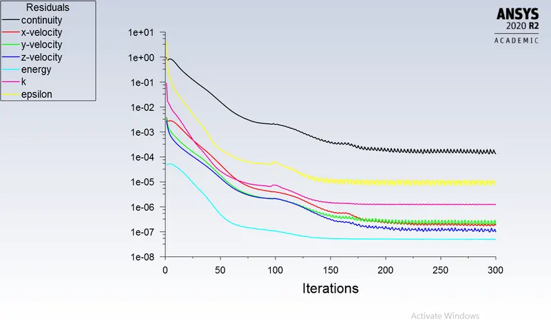
Since most fluid flow problems are of a non- linear nature, dealing with phenomenon like turbulence. to solve such problems we use an iterative solver to continuously improve our solution till 'convergence ' is reached. when solving a problem with multiple iterations convergence becomes related to the accuracy of the solution. typically when assessing convergence for a steady-state CFD solution we need to keep in mind three major things, they are:

1. Residual values
2. Solution Imbalance
3. Observing quantities of interest

the criteria for convergence that is being applied is:

1. continuity
2. x- velocty
3. y- velocity
4. z-velocity
5. energy
6. turbulence related variable

Y+:

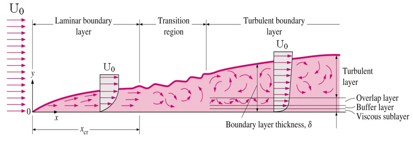
y+ is a non dimensional term that is used to define how fine or course the mesh is, This helps us determine if we need to use specific wall function.

1. uτ is the so called friction velocity
2. y is the absolute distance from the wall
3. ν is the kinematic viscosity

when we consider a boundary layer, there exist 2 regions the inner boundary layer and the outer boundary layer. The inner boundary layer consists of 3 main regions, the first is the viscous region which is right after the wall, in this region the viscous forces dominate the interial forces and the flow is laminar(y+ <10). The next is the transition region(10 < y+ < 30 ) and the third is the turbulent boundary layer, here the inertial forces are more dominant(30 < Y+ <300). The y+ value helps us decide the type of turbulence model that we need to use for the perticular problem.

turbulence models:

Reynolds averaged navier stokes equation:

The Reynolds-averaged Navier–Stokes equations (or RANS equations) are time-averaged equations of motion for fluid flow. The idea behind the equations is Reynolds decomposition, whereby an instantaneous quantity is decomposed into its time-averaged and fluctuating quantities.The RANS equations are primarily used to describe turbulent flows. These equations can be used with approximations based on knowledge of the properties of flow turbulence to give approximate time-averaged solutions to the Navier–Stokes equations.

1) k-Epsilon:

K-epsilon (k-ε) turbulence model is the most common model used in Computational Fluid Dynamics (CFD) to simulate mean flow characteristics for turbulent flow conditions. It is a two equation model that gives a general description of turbulence by means of two transport equations (PDEs). The original impetus for the K-epsilon model was to improve the mixing-length model.In the k–ε model the kinematic eddy viscosity νt is expressed as the product of a velocity scale ϑ = k and a length scale l= k3/2/ε. The rate of dissipation of turbulence kinetic energy ε is not the only possible length scale determining variable
Realizable k- ε Model: An immediate benefit of the realizable k-ɛ model is that it provides improved predictions for the spreading rate of both planar and round jets. It also exhibits superior performance for flows involving rotation, boundary layers under strong adverse pressure gradients, separation, and recirculation. In virtually every measure of comparison, Realizable k-ɛ demonstrates a superior ability to capture the mean flow of the complex structures.

2)k- omega:

In computational fluid dynamics, the k–omega (k–ω) turbulence model is a common two-equation turbulence model, that is used as an approximation for the Reynolds-averaged Navier–Stokes equations (RANS equations). The model attempts to predict turbulence by two partial differential equations for two variables, k and ω, with the first variable being the turbulence kinetic energy (k) while the second (ω) is the specific rate of dissipation (of the turbulence kinetic energy k into internal thermal energy).
The k–ω model initially attracted attention because integration to the wall does not require wall-damping functions in low Reynolds number applications. The value of turbulence kinetic energy k at the wall is set to zero. The frequency ω tends to infinity at the wall, but we can specify a very large value at the wall.apply a hyperbolic variation ωP = 6ν/(β1 y^P/2) at the near-wall grid point. Practical experience with the model has shown that the results do not depend too much on the precise details of this treatment.

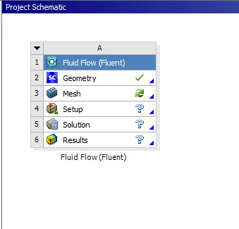
Procedure

1. To extract volume open space claim, under prepare menu use volume extract command and select the edges of the geometry and suppress the uploaded step file.

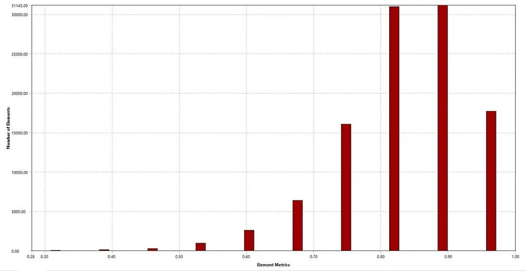
2. Open the mesh window and enter the mesh parameters and generate the mesh and also check for quality of the mesh which should not be less than 5%. Update the mesh window at the end

3. Open the setup window to select the turbulent models and enter the initial and boundary conditions under physis menu.

4. To plot the graph of weighted average temperature and standard deviation we need to define it in definitions under solutions window.

5. Initialze the model under use defined menu to calculate the values for initial time step and then enter the number of iterations to perform.

Preprocessing

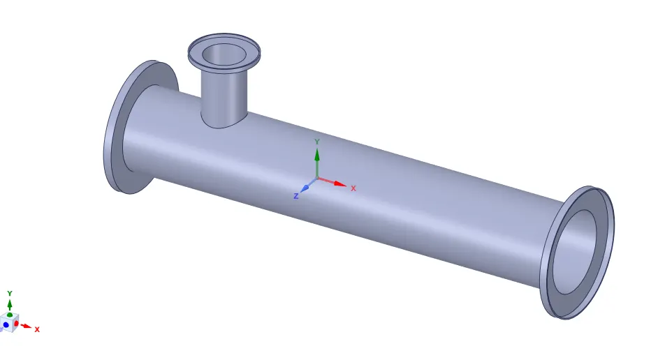
Imported Geometry

In this, We imported the geometry(Tee-shape tube) in Space-claim, where the geometry was in raw state as created in CAD package software. Here, We have represented the geometry in trimetric view given below:-

Cleaned up geometry in Space-claim

Since Geometry was in solid state where the body was having thickness which need to be remove so as to make geometry simple and can be converted into volumetric form. The newly updated geometry in volumetric form was as given below,

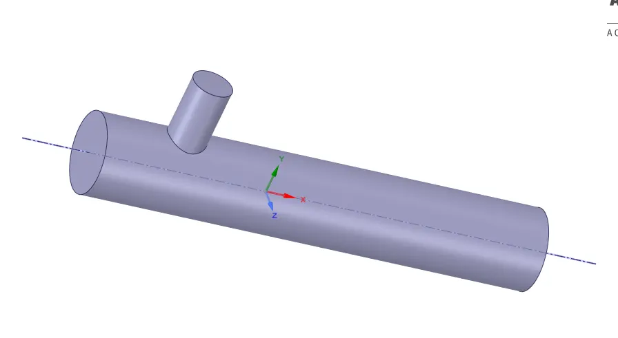
Meshed geometry in Ansys Mesher

Here, We imported the volumetric geometry created in Space-claim after cleaning up the geometry. Here, we applied meshing on the volumetric region with base mesh size. We also make sure that mesh quality should be of good quality.

After importing 3D cad geometry in ansys mesher the first step is to name the boundries by selecting the surfaces and rt clicking and slecting "Create Name Selection" or just by click N on the selected surface. There are two inlets i.e X-inlet which is along the X- axis (as shown in geometry) and other inlet is perpendicular it called Y- Inlet and the other end of pipe is Outlet. After this the element size is provided and mesh is created.

The created mesh is using element type as tetrahydral mesh in this study which is unstructured type of mesh.

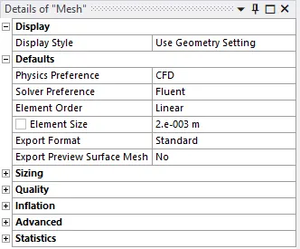
Meshed model with mesh cell size of 2mm.

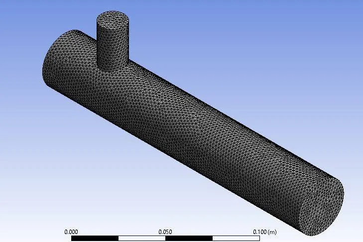
No. of cells = 105836

Nodes = 21342

Mesh quality:

Solving / Setup

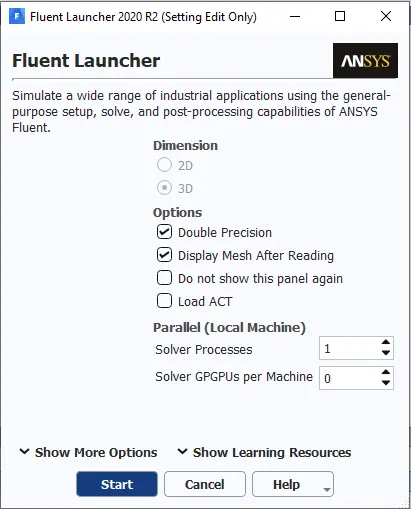
Ansys Fluent is used as the solver. Here, We have created the setup for simulation where we have provided double precision and displayed mesh after reading so that We can visualize the mesh obtained in design moduler.

Single precision means that the floating point numbers will be represented in 32 bit system whereas double precision means that they will be represented in 64 bit system. So Calculation in double precision will be more accurate. Though the performance of CPU takes a hit as it takes longer solution time for solving 64 bit floating point numbers as well the solution requires more RAM to store those nos.

A steady state computational study has been performed using a pressure based solver. Air was used as the fluid entering from both the inlets. The default physical properties defined in Fluent were used.

Selecting boundary markers shows that what are the inlets and outlet. Blue Colours arrows shows inlet and red colour shows outlet.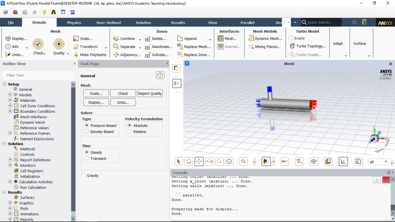

Turbulence Model

RANS based two turbulence models are used to analyze the mixing effectiveness of the mixing tee.

1. K-epsilon realizable Turbulence model with standard wall function

An immediate benefit of the realizable k-ɛ model is that it provides improved predictions for the spreading rate of both planar and round jets and captured turbulence in the bulk flow. While wall function added here which capture the information near the wall.

Pros: Robust, Easy to implement. Valid for fully turbulent flows only. Suitable for bulk flow, initial screening of alternative designs, and parametric studies.
Cons: Performs poorly for complex flows involving severe pressure gradient, separation, strong streamline curvature. And wall shear stress overestimated by wall function so that delay in separation occurs. Another shortcoming is numerical stiffness when equations are integrated through the viscous sublayer which is treated with damping functions that have stability issues.

2. SST K-Omega Turbulence Model
Shear Stress Transport (SST) is a variant of the standard k–ω model and used when there are wall effects present within the case.
Pros: The SST model accounts for the transport of turbulent shear stress and gives highly accurate predictions of the onset and the amount of flow separation under adverse pressure gradients. SST is recommended for high accuracy boundary layer simulations.
Cons: Dependency on wall distance makes this less suitable for free shear flows compared to standard k-w. It requires mesh resolution near the wall.

Boundary conditions - Momentum ratio of 2 and 4 have been used in the study. The hot stream enters in the main pipe (larger diameter) while the colder stream enters from the secondary inlet.

Table 1. Boundary conditions

	Velocity of hot air stream (m/s)	Velocity of cold air stream (m/s)	Temperature of hot air stream (oC)	Temperature of cold air stream (oC)
Case 1	3	6	36	19
Case 2	3	12	36	19

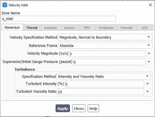
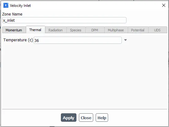
(i) Inlet velocity for x -axis :-

Here, We have given value of velocity for x-axis 3 m/s and gauge pressure 0 Pa and value for all other parameters have been taken default.

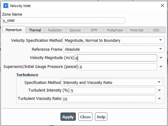
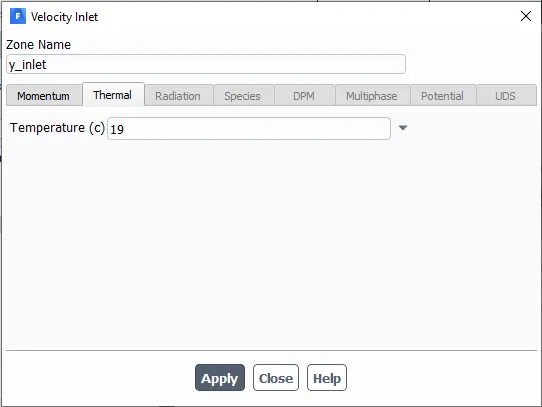
(ii) Inlet velocity for y -axis :-

Here, We have assumed value of velocity for y axis 6 m/s and gauge pressure 0 Pa whereas value for all other parameters have been taken default.

(iii) Wall condition for pipe :-

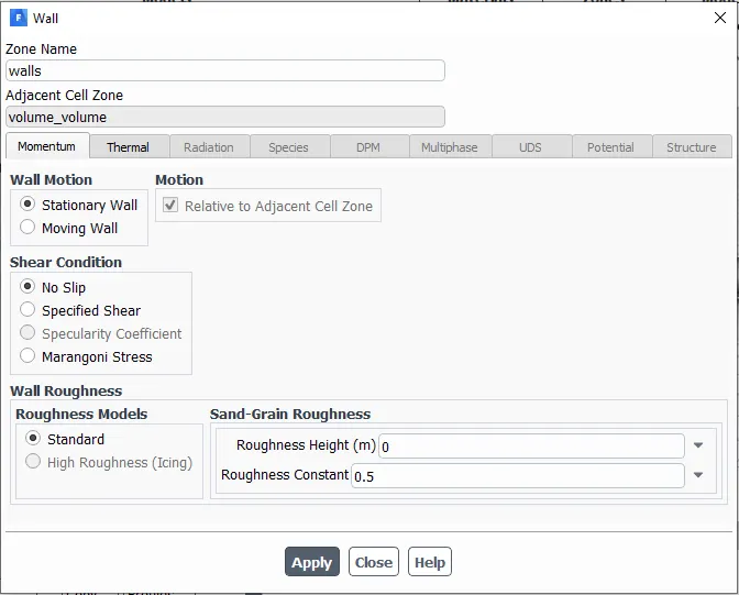
Wall conditions have been taken in the following way :-

• Stationary wall motion
• No Slip condition for shear stress
• Standard Roughness Model have been assumed at the surface
• Other parameters have been default value

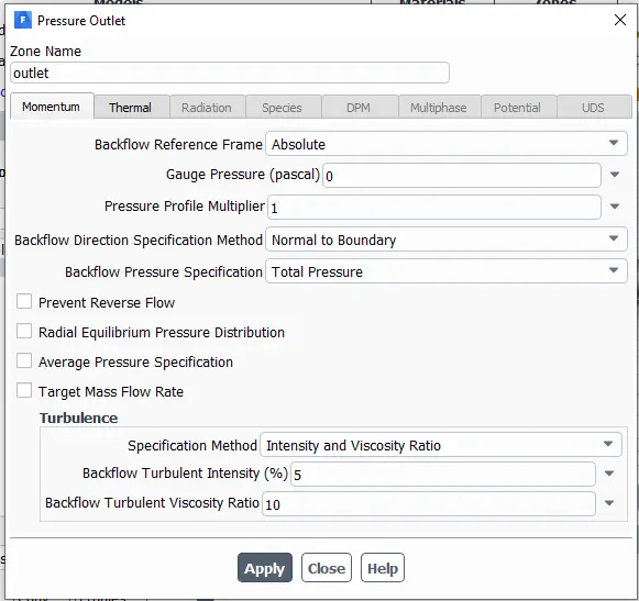
(iv) Outlet condition for pipe :-

Here, values have been assumed by default for all the conditions.

the results of the k–ε model are much less sensitive to the (arbitrary) assumed values in the free stream, but its near-wall performance is unsatisfactory for boundary layers with adverse pressure gradients. This led to suggest a hybrid model using (i) a transformation of the k–ε model into a k–ω model in the near-wall region and (ii) the standard k–ε model in the fully turbulent region far from the wall, the ε-equation is transformed into an ω-equation by substituting ε = kω. this became the k–ω sst model.

With the above Initial and Boundary conditions simulation is done for K epsilon and K omega

Below are the plots for K-epsilon and K-omega for momentum ratio 2 for short Tee model.

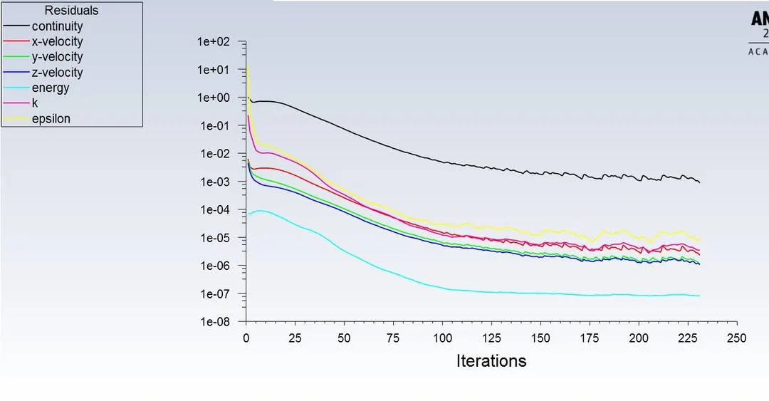
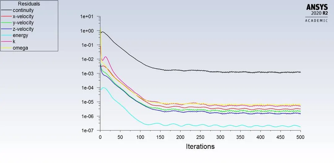
Residuals plots K epsilon

Residual plots for K-omega

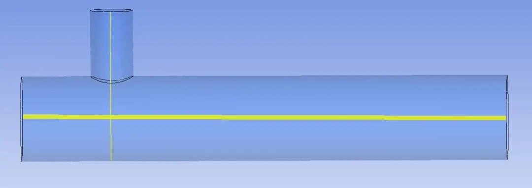
Line probe along length of the pipe and at the T junction.

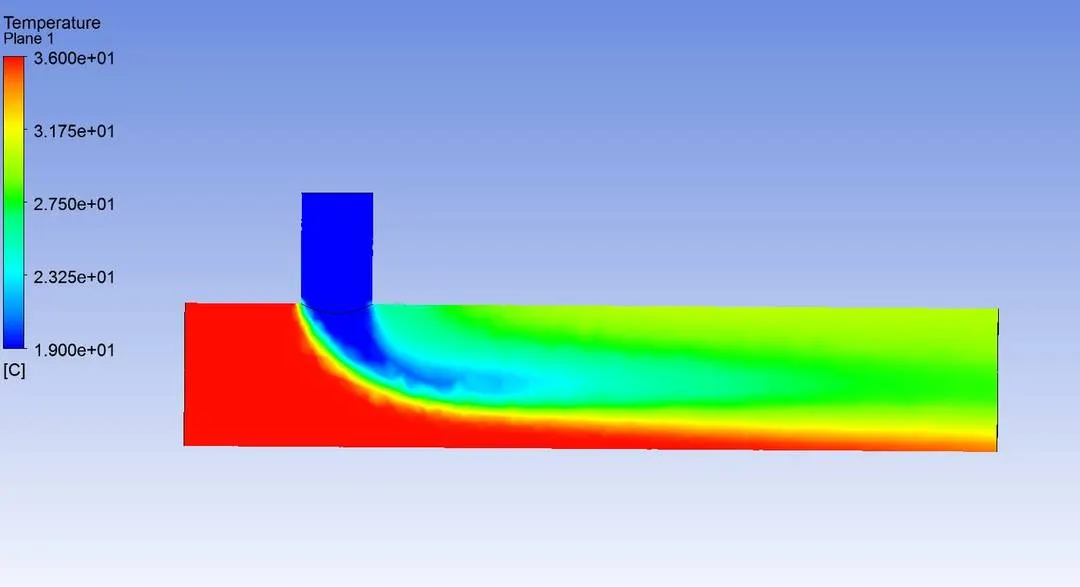
Temperature plot along the length using plane parallel to xy plane

K-epsilon

K-omega

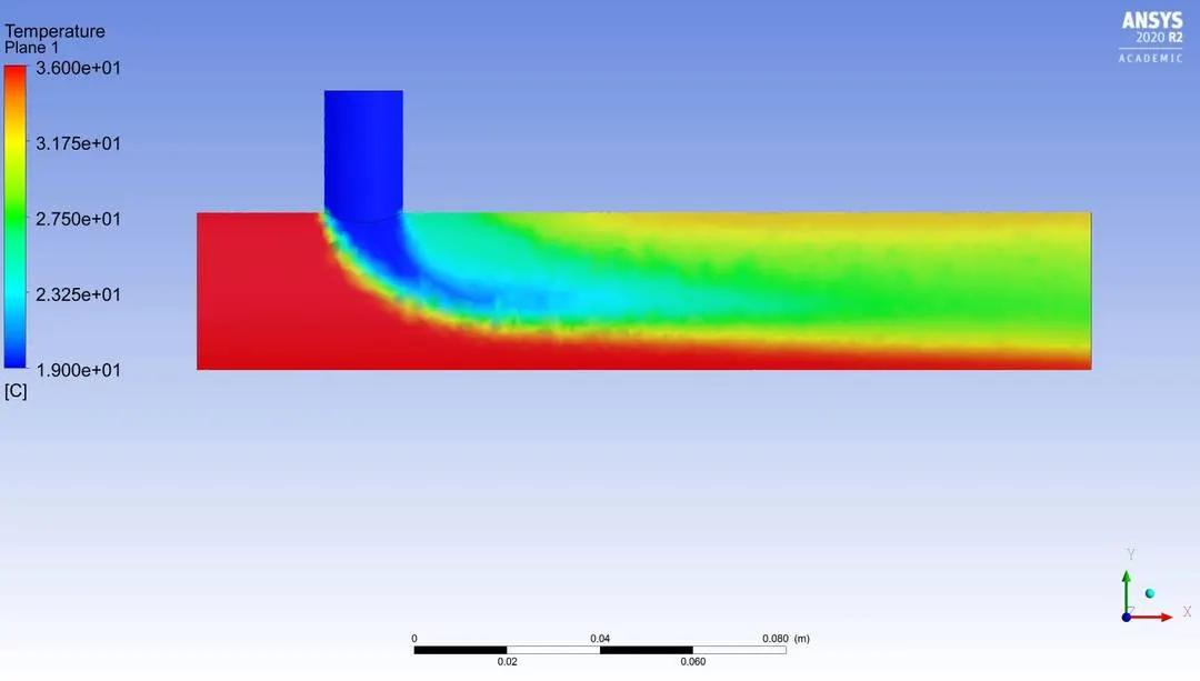
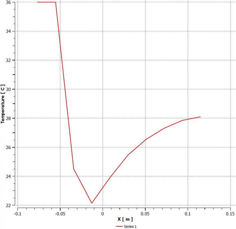
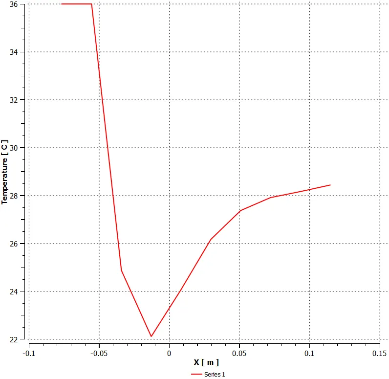
Temperature graph using line probe along the length

K-epsilon

K-omega

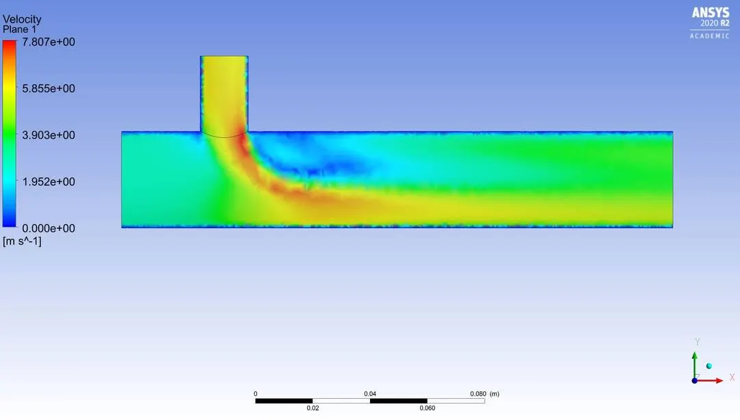
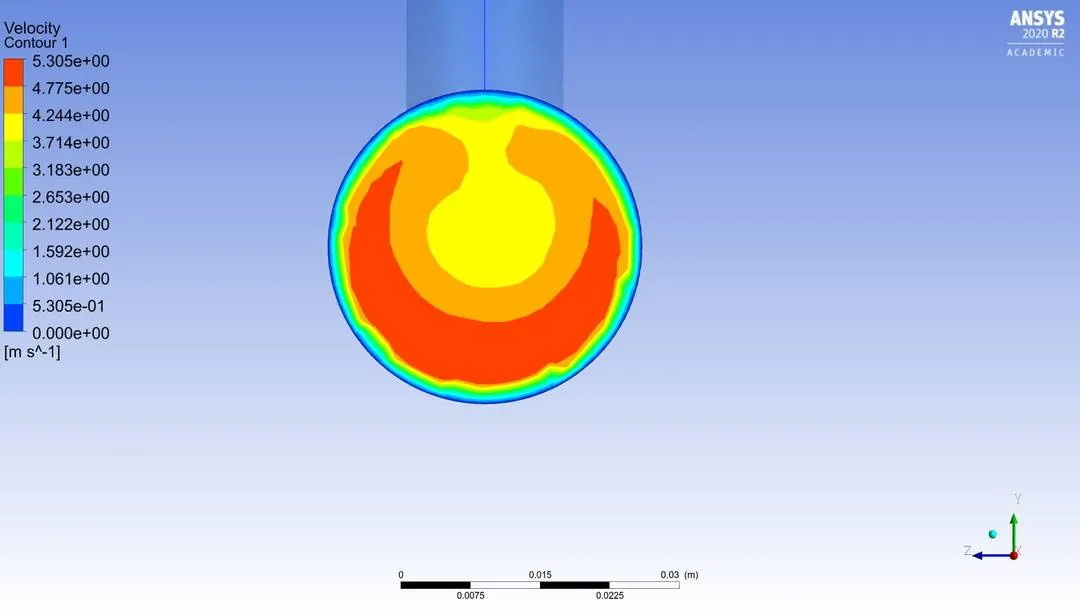
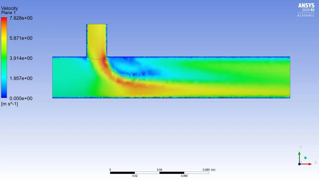
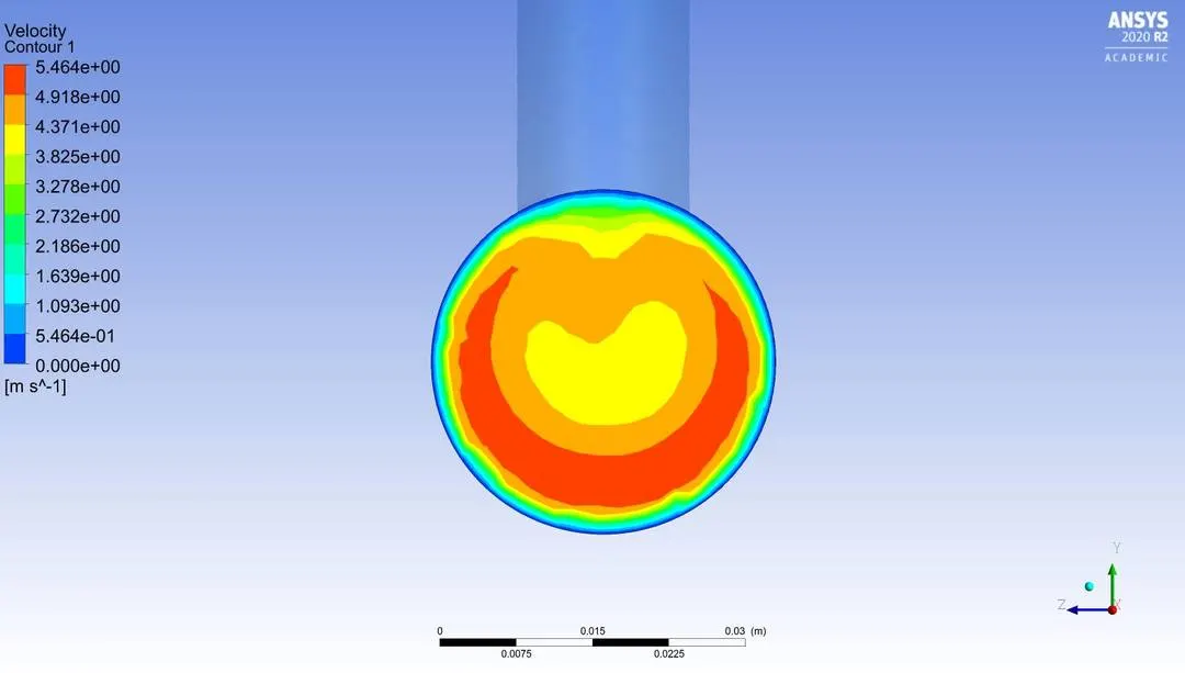
Velocity plot along the length using plane parallel to xy plane.

K-epsilon

K-omega

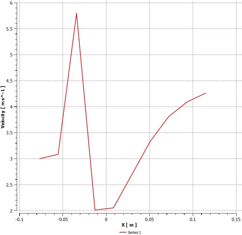
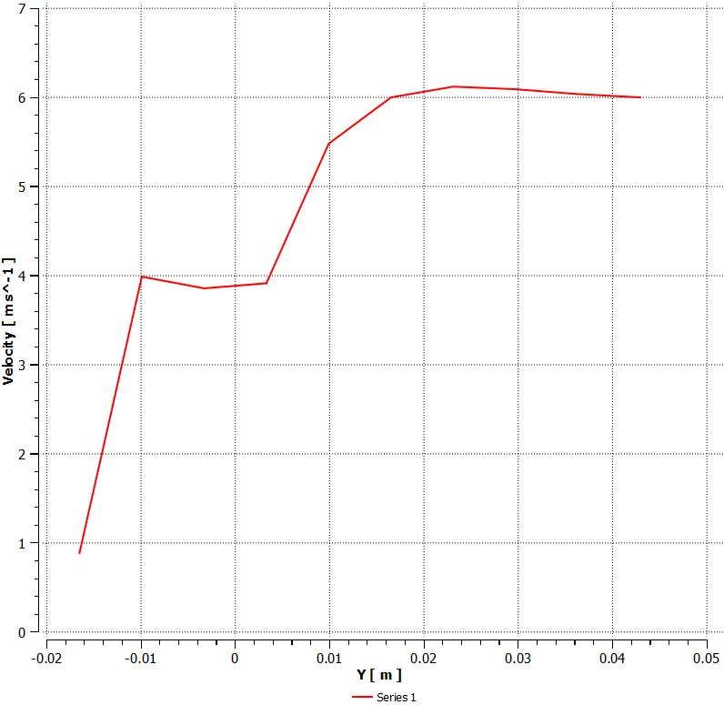
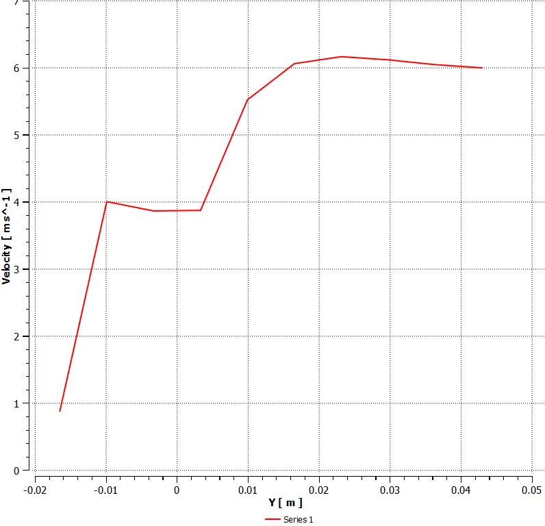
Velocity graph along the length using line probe.

K-epsilon

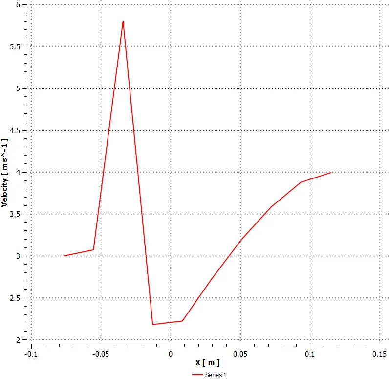
K-omega

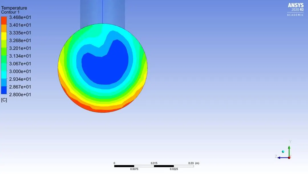
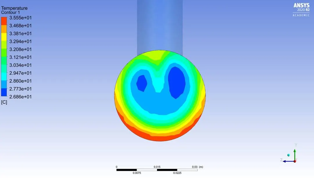
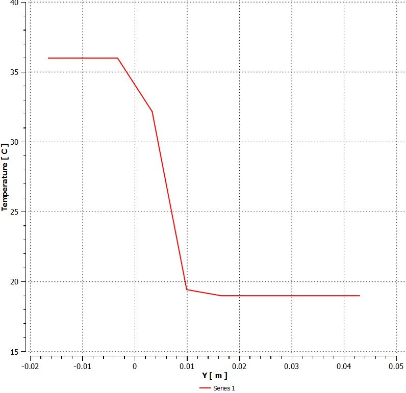
Temperature at T junction

K-epsilon.

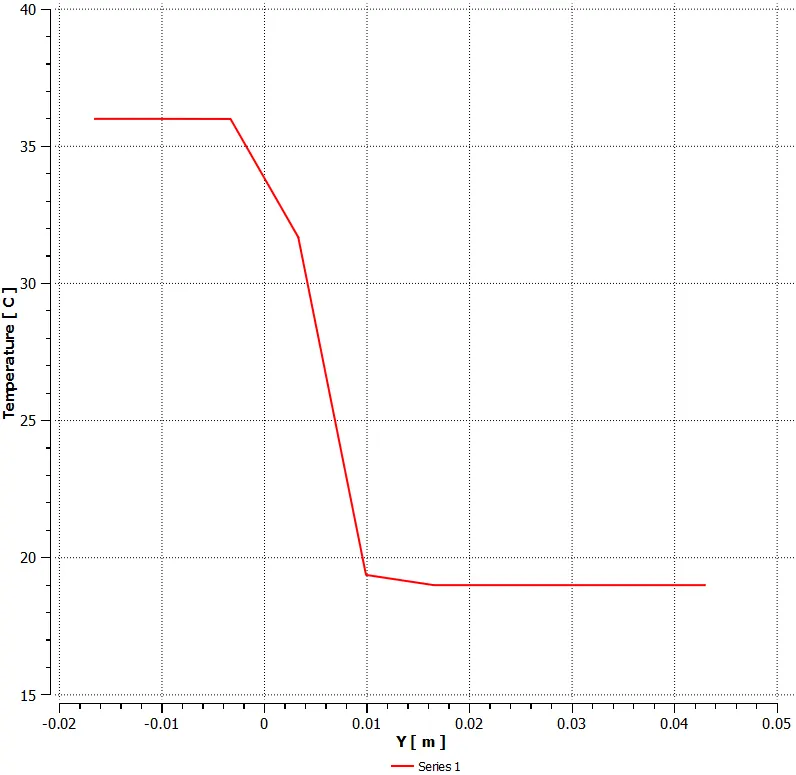
K-omega

Velocity at T junction

K-epsilon

K-omega

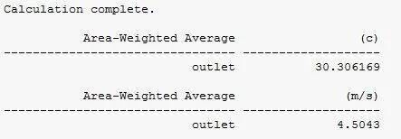
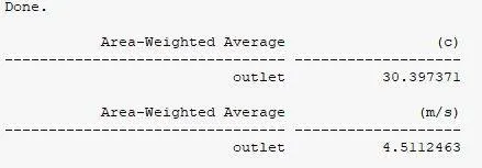
Weighted average values for temperature and velocity printed in console panel.

K-epsilon

K-omega

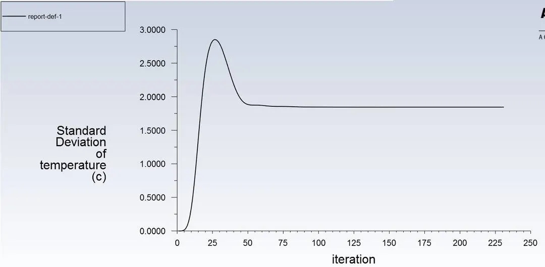
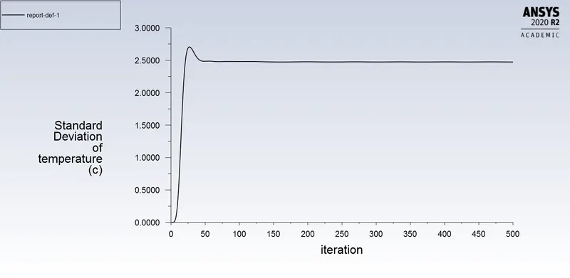
Standard deviation for temperature at outlet

K-epsilon

K-omega

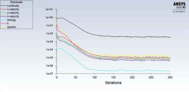
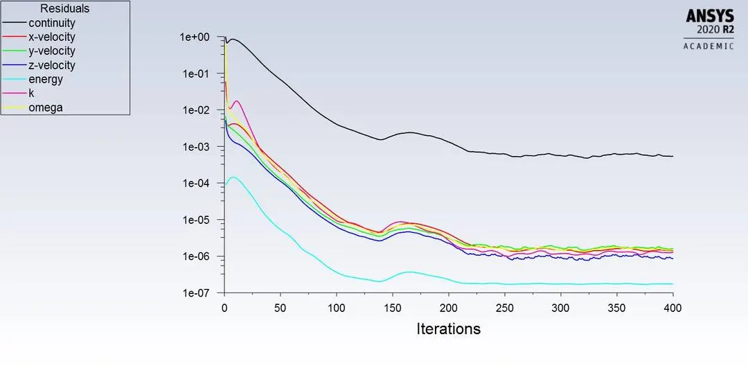
Simulation for momentum ratio 4 for short Tee model.

Residual plots

K-epsilon

K-omega

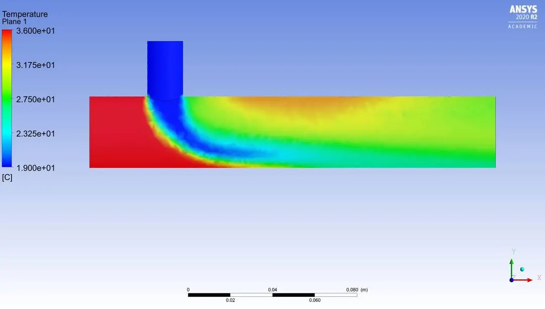
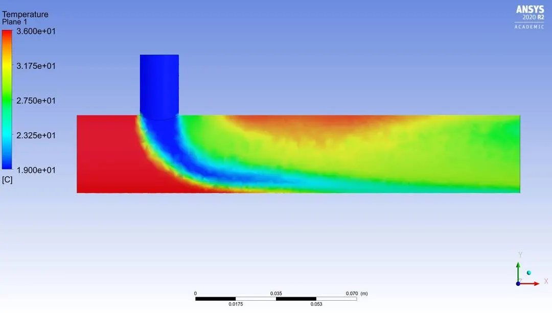
Temperature plot along the length

K-epsilon

K-omega

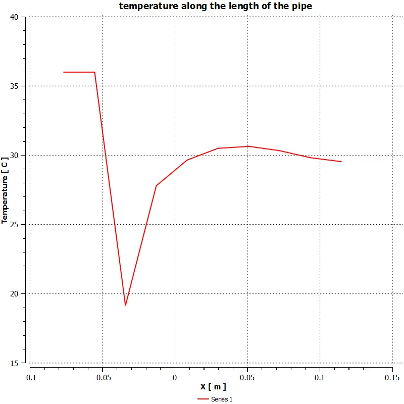
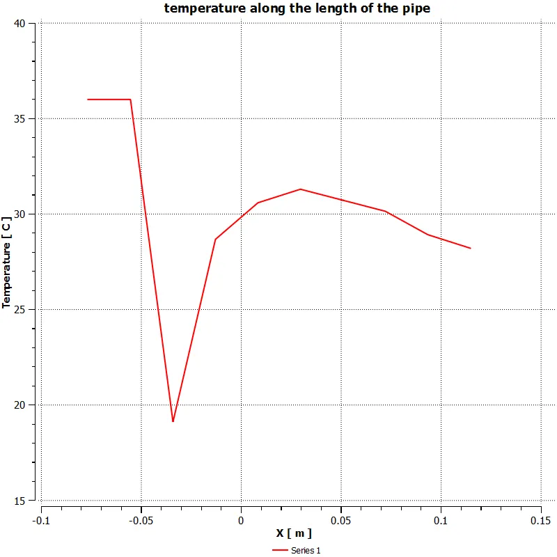
Temperature graph along the length

K-epsilon

K-omega

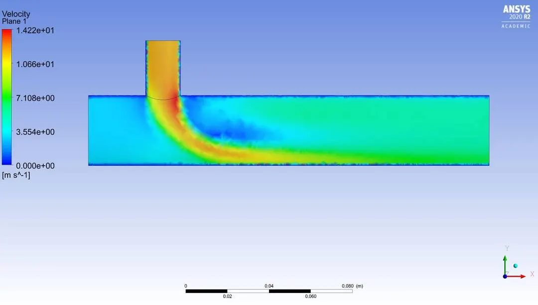
Velocity plot along the length

K-epsilon

K-omega

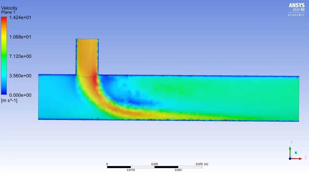
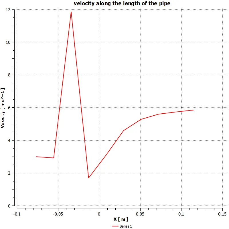
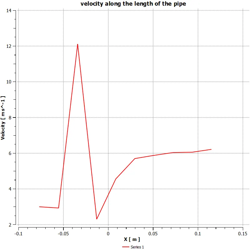
Velocity plot along the length

K-epsilon

K-omega

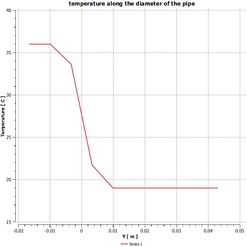
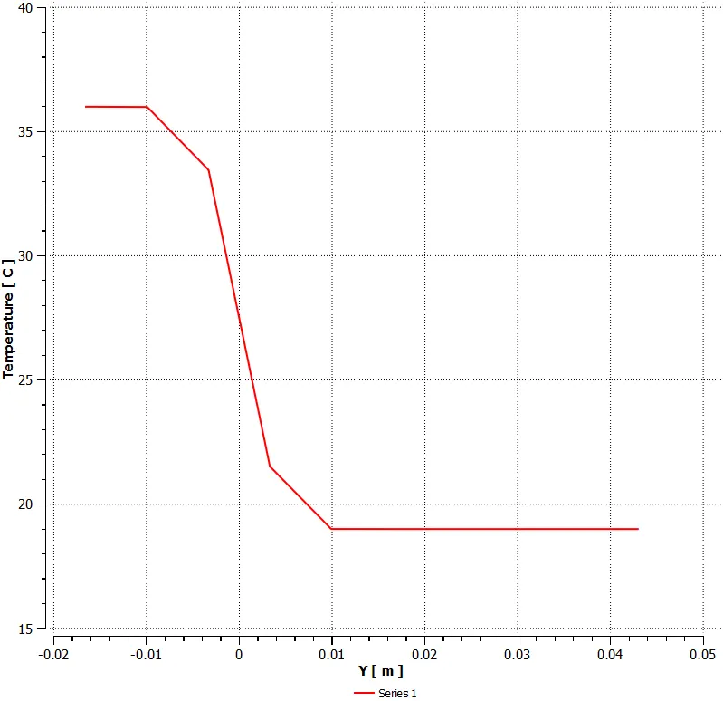
Temperature at T junction

K-epsilon

K-omega

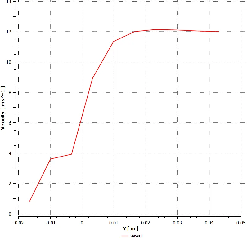
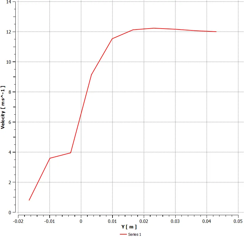
Velocity at T junction

K-epsilon

K-omega

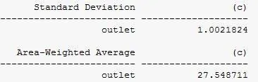
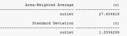
Weighted average values for temperature and velocity

K epsilon

K-omega

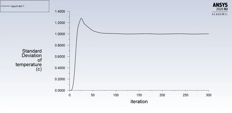
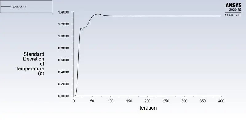
Standard Deviation of the outlet temperature

K-epsilon

K-omega

Inference:

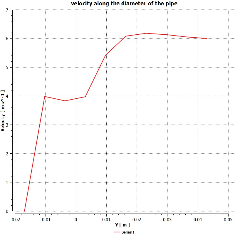
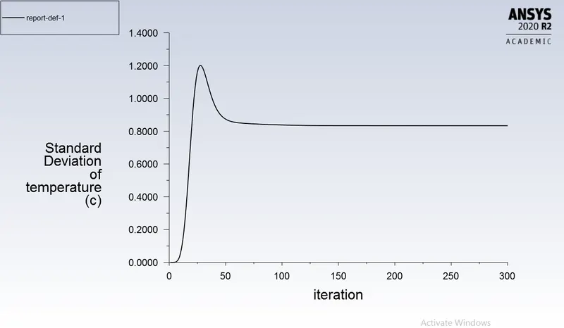
From the above plots we can infer that the converged solution varies in the order of 10−210-2 between K-epsilon and K-omega turbulent models and also the mixing efficiency is higher is K-epsilon model which is supported by Standard deviation plot, Higher the Standard deviation lower is the mixing efficiency and vice versa. From the residulas plots K-epsilon takes less no. of iterations when compared to K-omega model and also high Reynolds number is involved in which K epsilon results more accurate solution than K-omega and y+ values are above 5 which favors for K-epsilon turbulence models. Hence for this problem K-epsilon turbulent model is suitable.

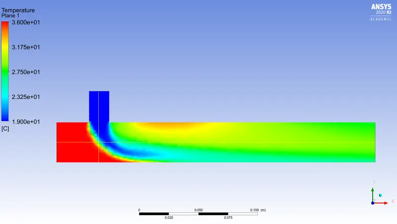
For momentum ratio 4, mixing efficiency is more which can be observed from the standard deviation plot (Higher standard deviation means low mixing efficiency and lower standard deviation means higher mixing efficiency) and the results obtained are closer to analytical solution.

Simulation for long Tee with momentum ratio 2 using K-epsilon turbulent model.

Residual plot

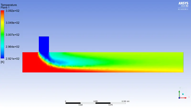
Temperature plot along the length

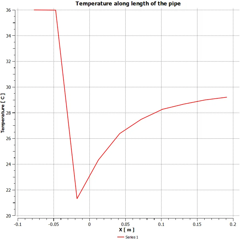
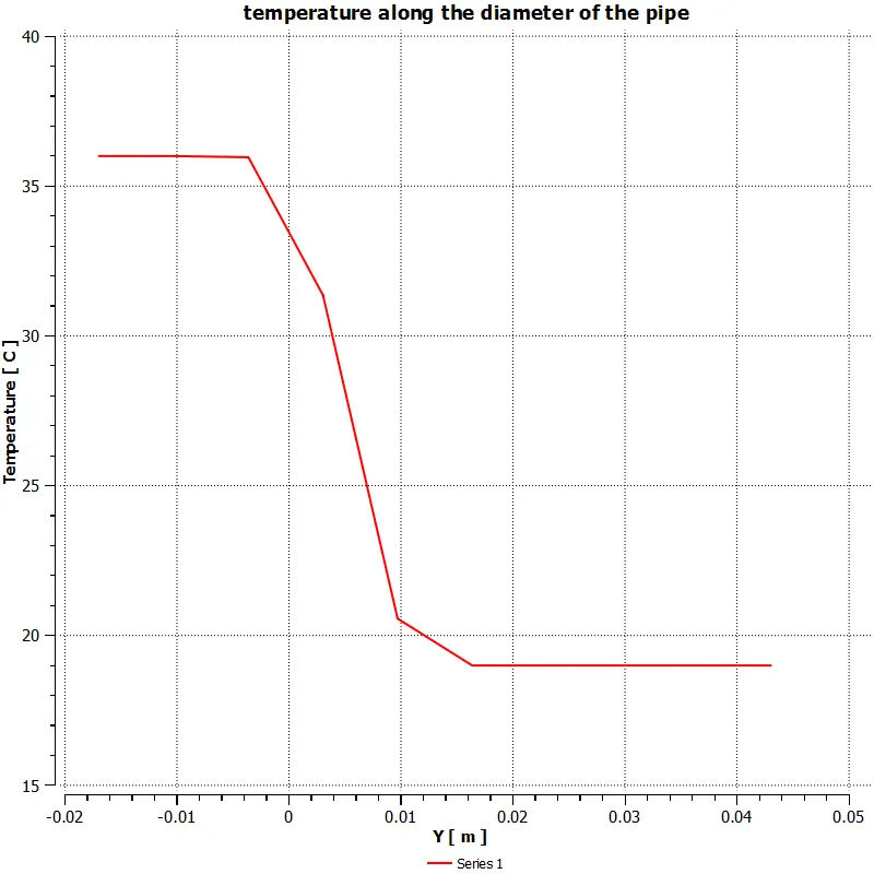
Temperature graph along the length

Velocity plot along the length

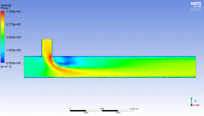
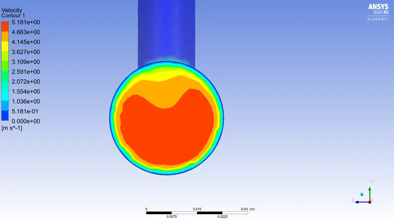
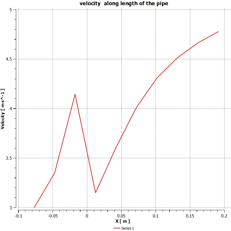
Velocity plot along the length

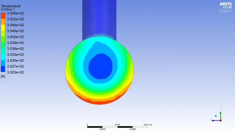
Temperature at the T junction

Velocity at the T junction.

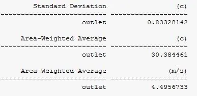
Weighted average values for temperature and velocity

Standard deviation for temperature at outlet

Simulation for long Tee with momentum ratio 4

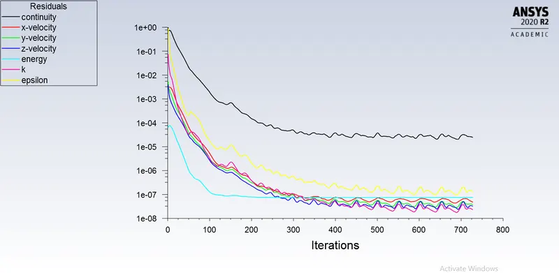
Residual plot

Temperature plot along the length

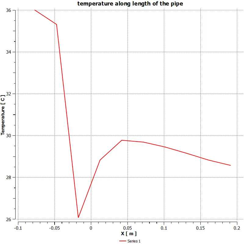
Temperature graph along the length

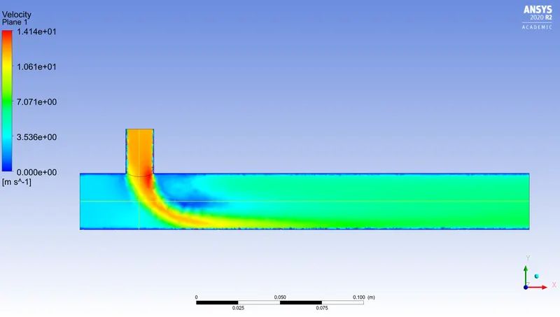
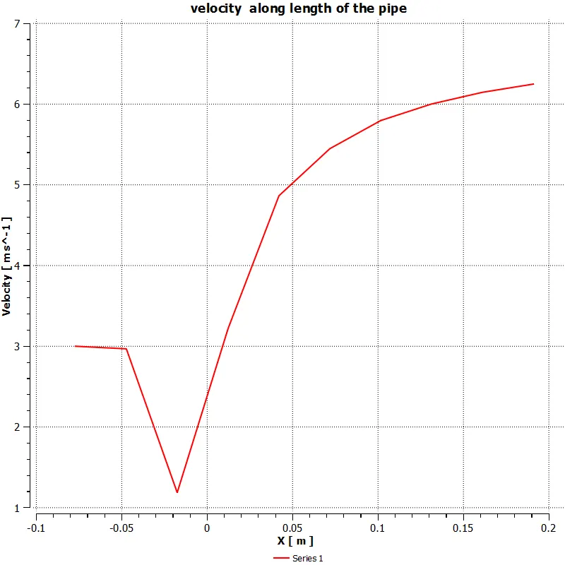
Velocity plot along the length

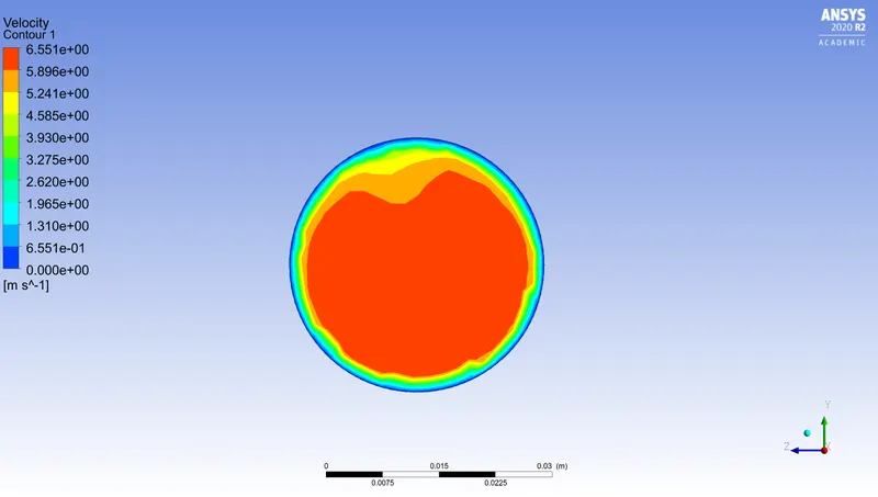
Velocity plot along the length

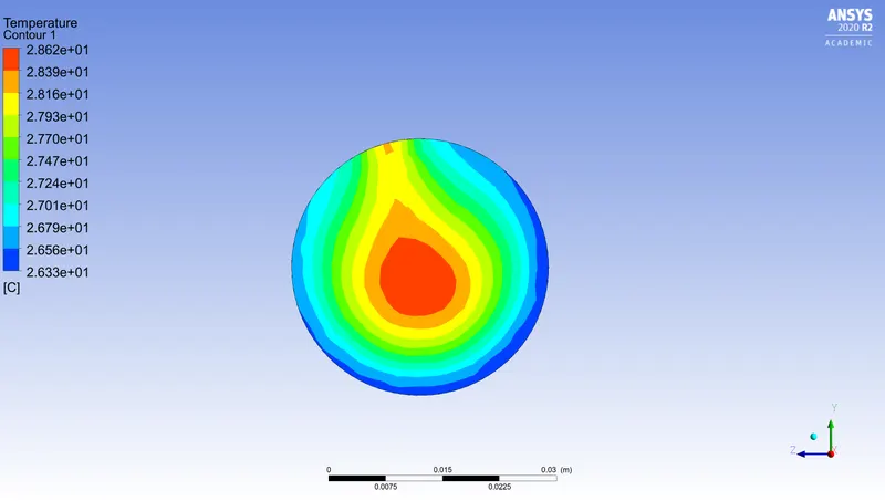
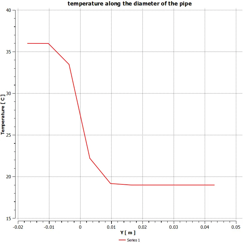
Temperature at T junction

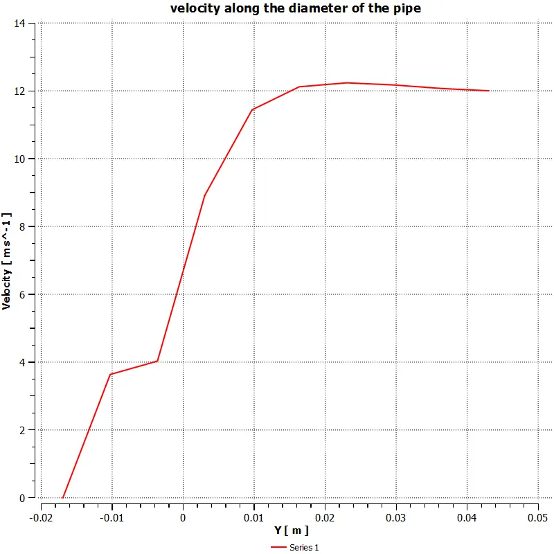
Velocity at T junction

Weighted average values for temperature and velocity

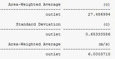
Standard Deviation at the outlet temperature.

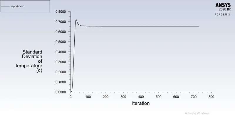
Table Comparing mixing efficiency of short tee and long tee model for K-epsilon turbulence model.

Model type	Momentum Ratio	Standard Deviation
Short Tee	2	2.25
Short Tee	4	1.0002
Long Tee	2	0.8
Long Tee	4	0.6

Inference:

From the above plots the variation of temperature and velocity for the given momentum ratio does not vary when compared with the short Tee. However from standard deviation at the outlet temperature decreases indicating higher mixing efficiency with increase in length.

Grid Independence test

In order to verify that the results obtained from the simulation do not vary with size of the mesh, no. of mesh cells are varied by increasing the mesh element size.

Type	Turbulence model	Mesh cell size	Cell Count	Y+ range	Weighted Average outlet temperature (celius)	No. of iterations
Short Tee with momentum ratio 2	K-epsilon	1.5mm	211968	4-14	30.35	280
		2 mm	105836	6-16	30.30	230
		5 mm	14330	10-30	30.27	200

From the above table we can observe the y+ value range increases as the mesh cell size increases because of which K-epsilon turbulent models results more accurate solution which can be seen from the average temperature values at the outlet of the tee model.

Comparison of all case setups

Case Type	Turbulence Model	Cell count	Standard Deviation	Average Outlet Temperature	Iterations For convergence
Baseline simulation (Short Tee)	Realizable K - epsilon	14,202	1.5	30.25	300
short Tee ( Momentum ratio 2)	Realizable K - epsilon	509336	1.5	30.25	125
Short tee ( Momentum ratio 2)	K Omega SST	509336	1.6	30.30	300 - 350
Short tee ( Momentum ratio 4)	Realizable K - epsilon	509336	1.2	27.5	300 - 350
Long tee( Momentum ratio 2)	Realizable K - epsilon	510936	1.25	30.35	139
Long tee ( Momentum ratio 4 )	Realizable K - epsilon	510936	0.7	27.5	300 - 350

Conclusion:

The resultant average temperature for both turbulence model Reliazable K -Epsilon & K omega SST looks similar, but for computing K omega SST takes more time and more number of iterations for convergence. Moreover, K epsilon predicts far from the boundary and K omega capture well near the wall also for the simulation we are dealing with the wall. Because of this reason for the remaining case, I choose K - Epsilon Turbulence model.

For both case momentum ratio of 4, the outlet temperature drops significantly this occurs because of very high cold velocity air. So this clearly shows higher the momentum ratio greater the efficiency of the tee.

We are getting an almost similar result for short tee & long tee for the momentum ratio of 4 from this we can get to know that the length of the pipe doesn't affect the efficiency of the pipe.

When it comes to standard deviation, the long tee gives very lower value compared to the short tee. Indeed, we can increase high inlet cold air velocity for the application so we can get pretty good mixing in nature for a short pipe instead of using the long pipe.

Overall, the short tee pipe gives a pretty good result, and also it saves material cost. Increasing the pipe length doesn't create any difference in the outlet temperature.