Roof Crash Analysis of a Neon Car Model using Hypermesh and RADIOSS

Objective

set up a Neon car model and perform a roof crash analysis using Hypermesh and solve the model using RADIOSS solver.

In this project, we will be setting up the case for roof crash analysis for a reduced neon car model.

Step 1 - Geometry manipulation

Step 2 - Contact Definition

Step 3 - Apply Boundary Conditions and Run the Simulation

Step 4 - Post Processing using HyperView and HyperGraph

Introduction

FMVSS 216 Roof Crush Resistance, establishes strength requirements for the passenger compartment roof of passenger cars, multipurpose passenger vehicles, trucks, and buses with a GVWR of 2722 kilograms or less. The purpose of the standard is to reduce deaths and injuries due to the crushing of the roof into the passenger compartment in rollover accidents.

The prescribed static loading device is a rigid unyielding rectangular block 762 millimeters in width and 1,829 millimeters in length. It shall not move more than 127 millimeters to achieve the specified resistive load when applied to the forward edge of a vehicle’s roof – see Figures 1 and 2. The resistive load to be achieved is 1½ times the unloaded vehicle weight (UVW) of the test vehicle or 22,240 Newtons, whichever is less.

Both the left and right front portions of the vehicle's roof structure shall be capable of meeting the requirements but a particular passenger car need NOT meet further requirements after being tested at one location. The passenger car's seats shall be placed on a rigid horizontal surface and fixed rigidly in position. The vehicle's windows shall be closed and the doors shall be locked. Any convertible top or removable roof structure shall be secured in place over the occupant compartment. Remove roof racks or other nonstructural components. The force shall be applied in a downward direction perpendicular to the lower surface of the static loading device at a rate of not more than 13 millimeters per second until reaching the compliant resistive load. The test shall be completed within 120 seconds. The static loading device shall be guided throughout the test so that it moves, without rotation, in a straight line with its lower surface oriented as follows and as shown in Figures 1 and 2.

1. Its longitudinal axis is at a forward angle (side view) of 5º below the horizontal and is parallel to the vertical plane through the vehicle's longitudinal centerline.
2. Its lateral axis is at a lateral outboard angle, in the front view projection, 25º below the horizontal.
3. Its lower surface is tangent to the surface of the vehicle.
4. The initial contact point, or center of the initial contact area, is on the longitudinal centerline of the lower surface of the static loading device and 254 millimeters from the forward most point of the centerline.
5. If the vehicle being tested is a multipurpose passenger vehicle, truck, or bus that has a raised roof or altered roof, and the initial contact point of the static loading device is on the raised roof or altered roof to the rear of the roof over the front seat area, the plate is positioned so that the midpoint of the rearward edge of the lower surface of the static loading device is within 10 mm of the transverse vertical plane located at the rear of the roof over the front seat area.

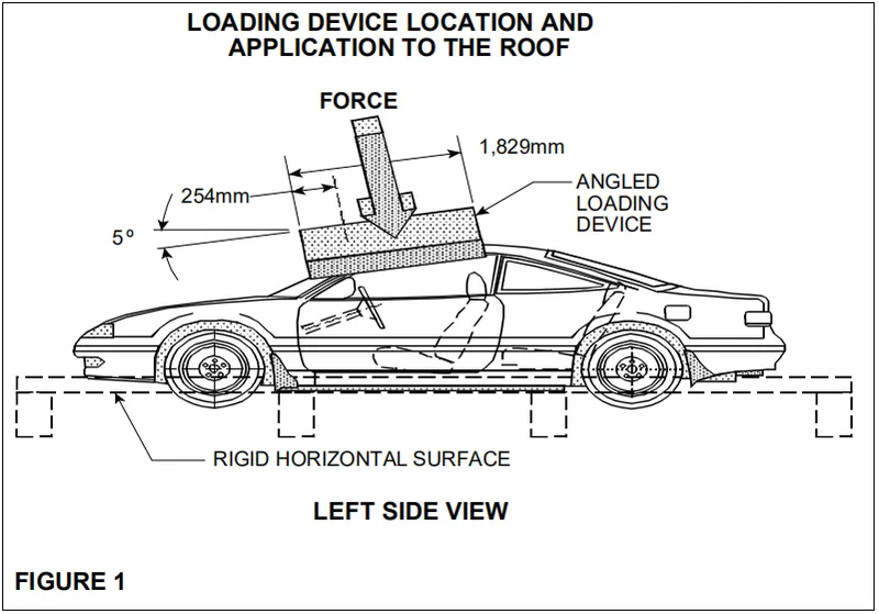
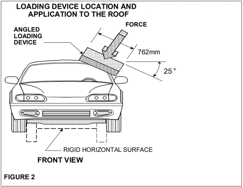
Real Roof Crush tests, quasi-static or dynamic, have been widely used to evaluate the safety integration of vehicle structure, where there are specific standards such as FMVSS 208 and 216. With the development of crash technologies, several crash solvers such as LS-DYNA3D, pam crash, and Radioss, are used for vehicle impact simulations. The most difficult of the simulation is still the quasi-static roof crush simulation. If a higher speed is used for the quasi-static simulation, it will result in inertia effects which smooth out non-linearities and deficiencies in the solution algorithms. While implicit solvers could address quasi-static impact scenarios, the large deformation of parts surrounding roof and pillar areas, and contact involving multiple vehicle parts make the convergence of the solutions very difficult and sometimes unstable within implicit solvers.

Quasi-static Analysis :

Static analysis is when the load does not depend on time. Dynamic analysis is when the load does depend on time and inertia plays an important role.

Quasi-Static, which is time-dependent but then the load acts at a slower rate such that the inertial effects of the body are negligible. When the body is loaded slowly its deformation rate is also very slow.

Procedure

Import the Model

In the data we have two files

Neon_roof_0000.rad and FMVSS_216_ROOF_IMPACTOR_coarse_0000.rad (starter input file): Which has all data required for the solver such as model information, elements, nodes, loads, boundary condition etc.

Neon_roof_0001.rad (engine input file): Which has all data required for the radioss engine i.e speed , time step, run time, what all data we want as output.

To import file,

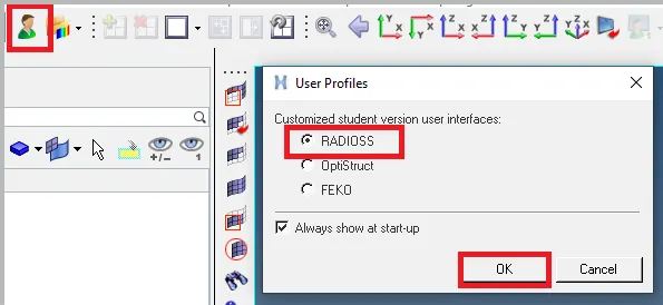
change user profile to radioss Because we are using solver as Radioss

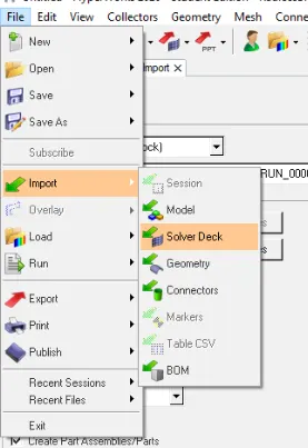
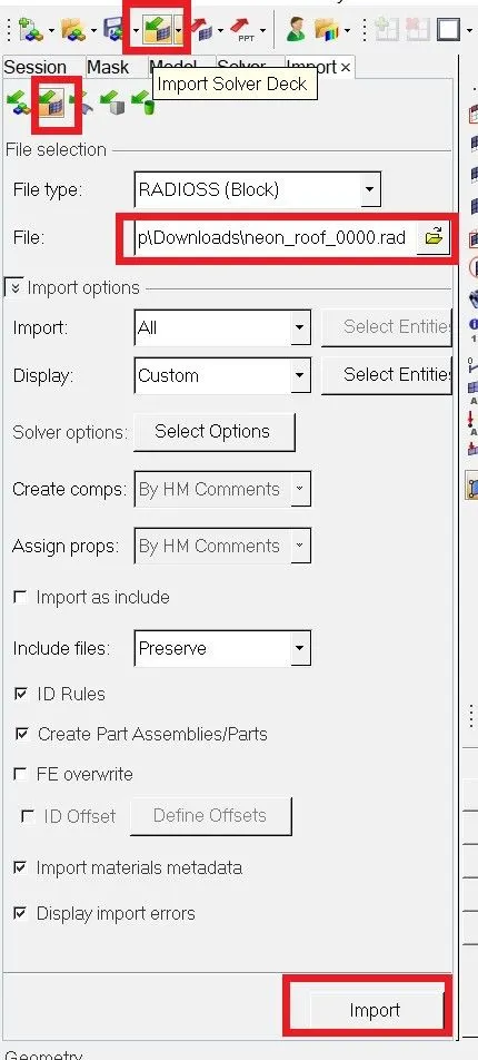
Go to File>Import>Solver deck. we can see the new tab where options available for browse file. Browse the starter input file,

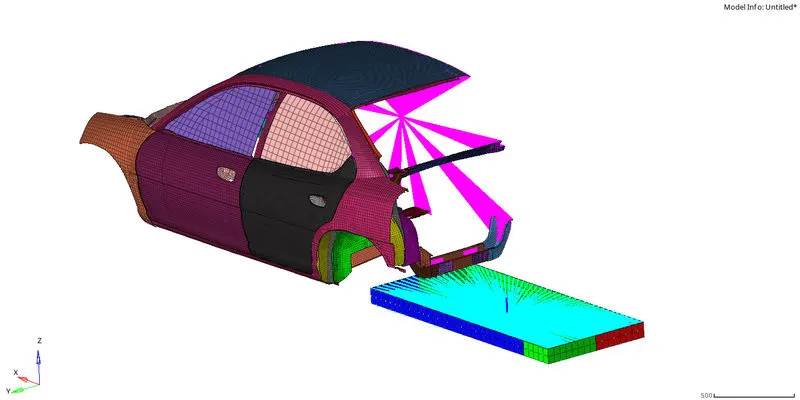
Reduced Neon Car Model

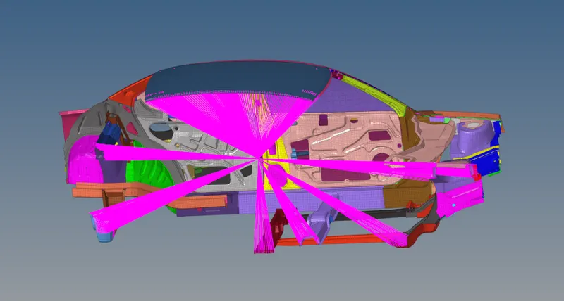
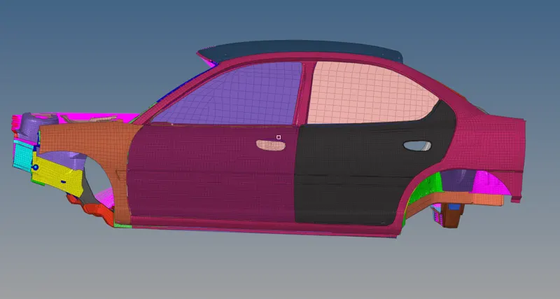
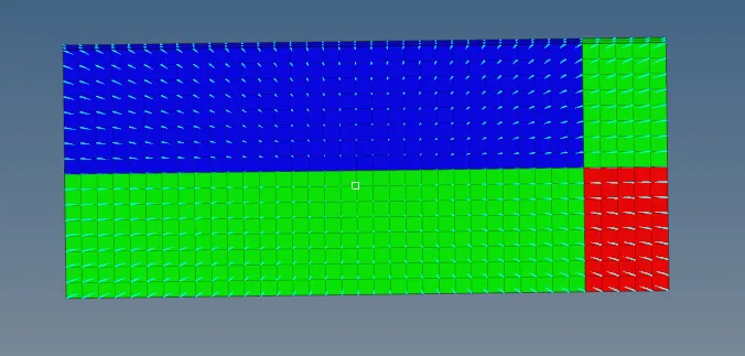
we also have to import the impactor separately

Impactor

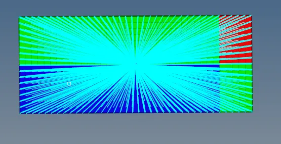
Car BIW and Impactor

Setting up the Solver

1) Check the unit system:

The very first step in the solver deck setup of this model is to check the units in which the Geometry has been modeled. To do this, we need to use the Begin card in the Model Browser as shown below. Here we can view the basic units of Mass, Length and time that were used in the model.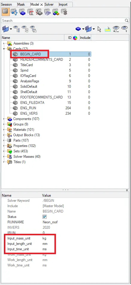

We can see that the units of Mass, Length and Time are Kg, mm, and ms respectively.

2) Positioning of the Impacter:

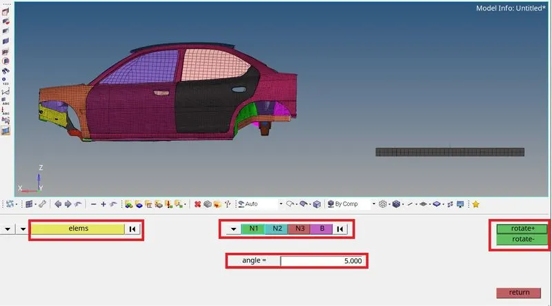
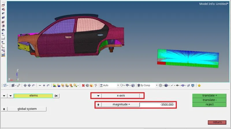
The next step is to position the Impactor at the desired location so that the Roof Crush simulation can take place appropriately. To do this, we simply need to use the rotate and translate command in the Tool Tab. Tool -> Translate and rotate command

We need to follow the steps in the order given below to position the Impactor at the right location:

1. A 180° rotation about the global z-axis with the point opposite to C as base point
2. A -5° rotation about the axis through axis AB
3. A 25° rotation about the axis through axis AC
4. A translation to put point A at global ( -3500.00, 584.822, 1343.06)

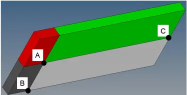
FMVSS 216 Impactor

Rotate command window

Translate command Window

After following these commands properly, we will get the impactor at the desired location as shown below: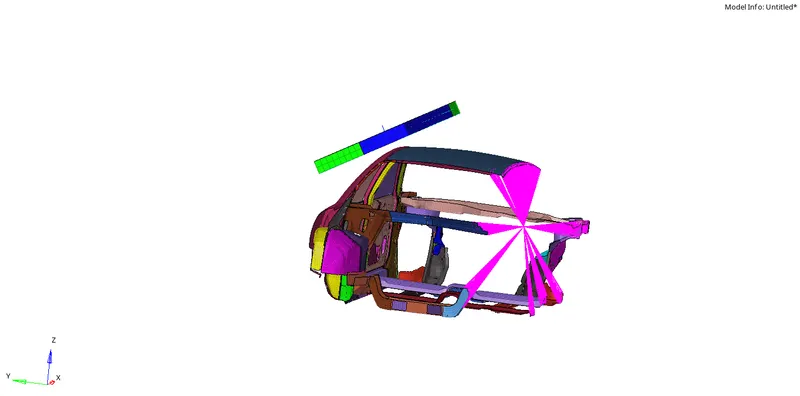

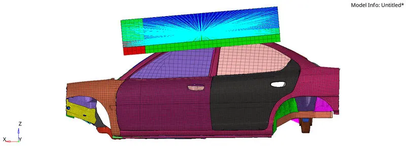
Final Positioning of the Impactor

some setups are done in HyperCrash and the remaining setups are done by Hypermesh.

CHECK FOR PENETRATION AND INTERSECTION:

This check was done using Hypercrash, To check penetration and intersection

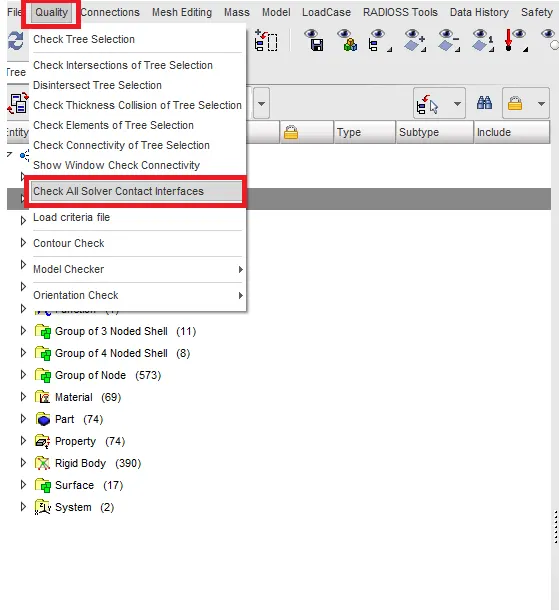
Got to Quality>> Check all solver contact interfaces >> Select parts > Click on check penetration

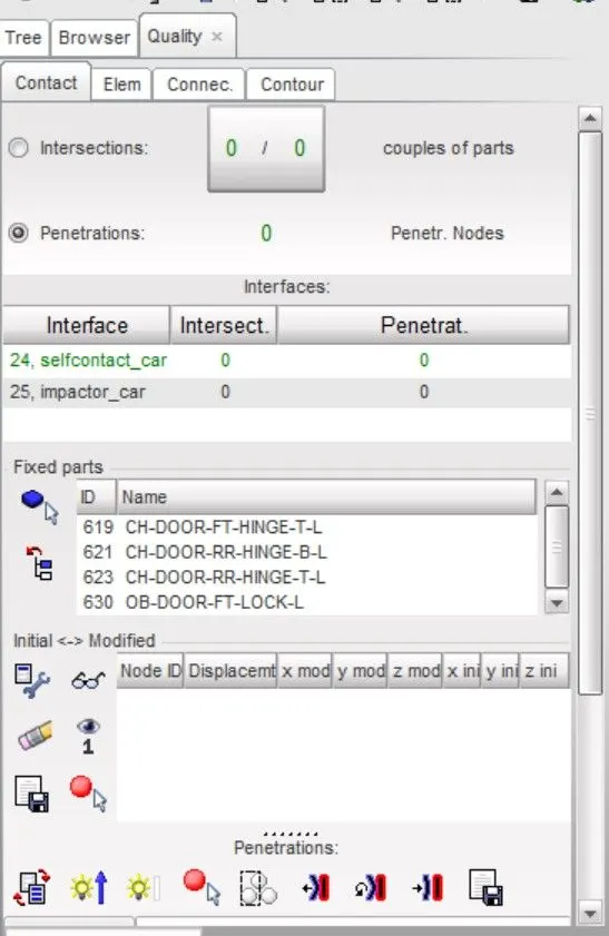
As you can see in the image below there are no penetrations or intersections present in the model

CREATING CONTACT INTERFACES

• Creating self contact

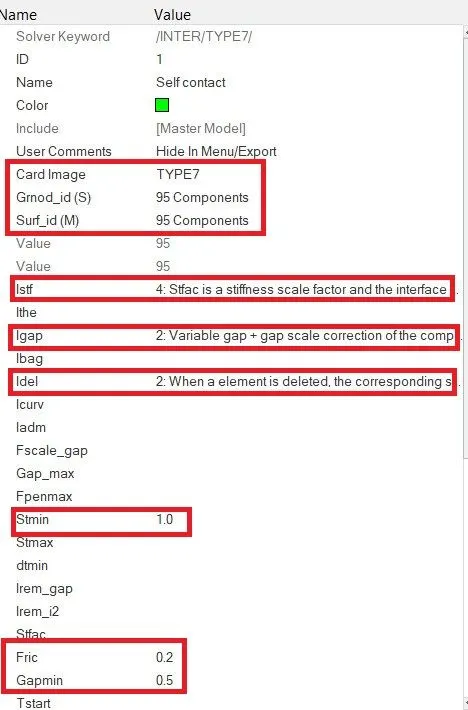
At first, we are defining a Type 7 self contact interface for the car model, When defining the Self impact contact, we will give the car model as both the slave and the master segment as we want to prevent the Car model from collapsing in itself. Since we have defined the slave and master as the car, the algorithm does not allow the master segment (car model) to penetrate the slave segment (car model), hence the self collapsing will not occur.

We will go to Solver browser and we will delete all the existing interfaces.

Now create a new contact

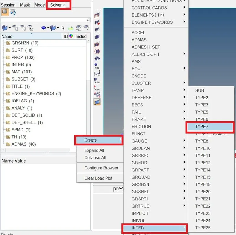
Goto Solver browser >> Right-click >> INTER >> TYPE 7

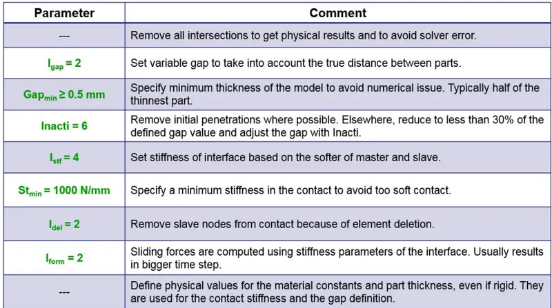
Recommended Properties for Type 7 contact Interfaces are as shown in below table

Self contact Type 7 card

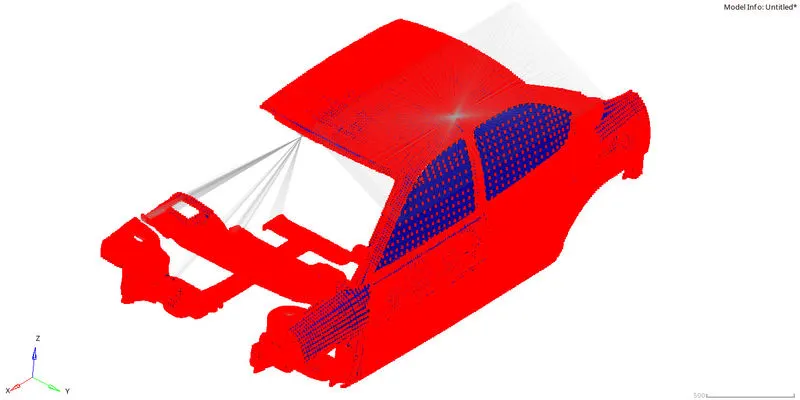
After creating self contact check whether master and slave nodes selected properly, For that, right-click on self-contact >> Review

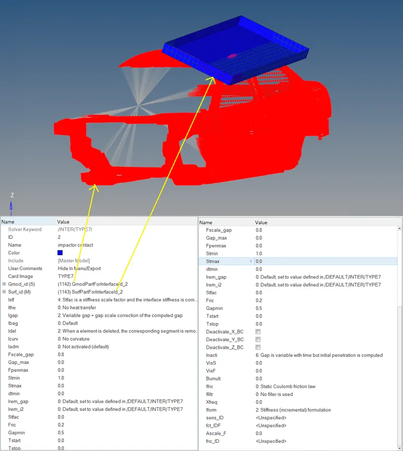
Contact Interface between Impactor and Car

Now we are going to create a Type 7 contact interface between car and impactor.

When defining the Contact between the Impactor and the car, the master segment will be the Impactor and the slave segment will be the Car model. This is because there is a much coarse mesh on the Impactor making the impactor much stiffer than the Car in this case. Also, the body under study is the car model and we want results and simulations for it, hence it is to be kept as the slave segment.

Output request from Contact interfaces

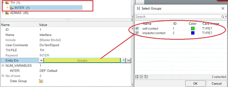
In order to get output results for post-processing, we need to create TH (Time History ) files for contact interfaces,

Solver browser -> right-click -> Create -> TH -> INTER

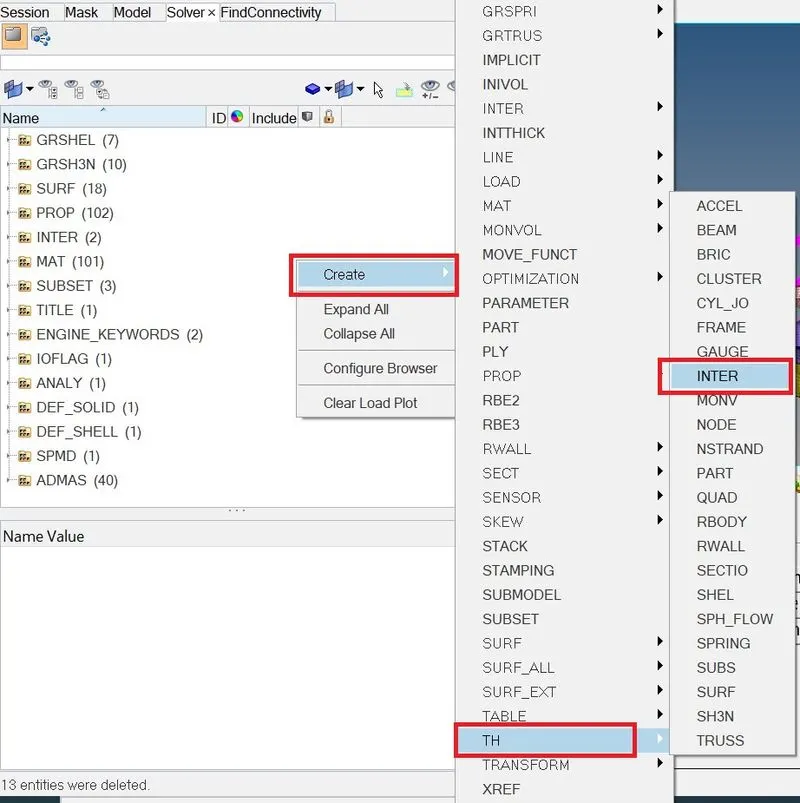
select the entities as the contact interfaces created, Refer to the image below:

Apply Boundary Conditions

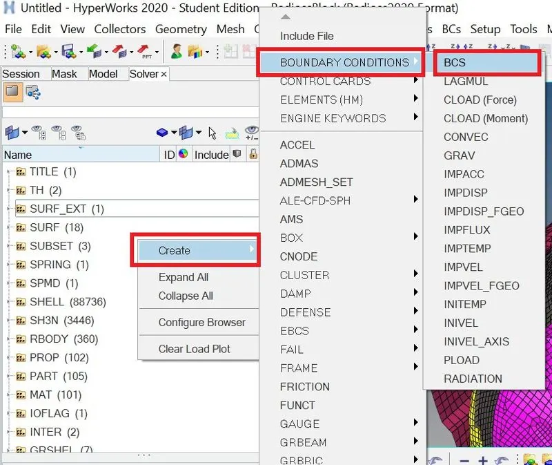
To create the Boundary conditions, right-click on the solver browser and use the Create option. In Create goto Boundary conditions -> BCS

Create Collectors to fix the suspension points of the car

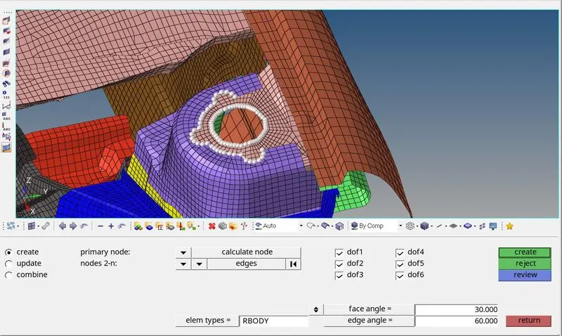
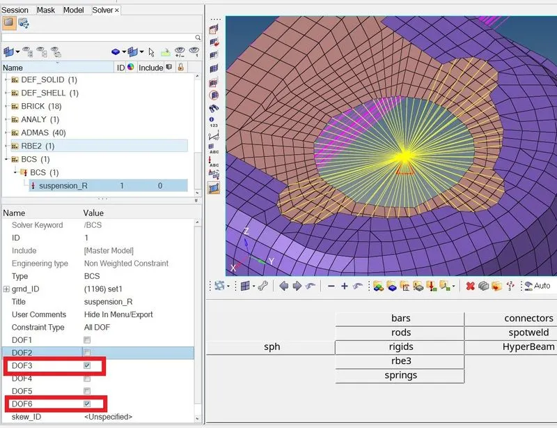
In order to keep the suspension shock tower nodes locked in Z direction, first, we need to create Rigid Body to connect the suspension shock tower nodes to a single Master node.Then we apply the Boundary condition for the Master nodes of the suspension.

Go to 1D-->Rigids -> Create and choose Calculated node option & Select edges on the Suspension shock tower hole in order to select the nodes and Click Create. As shown in figure below RBODY is created.

The reduced model has 3 suspension shock towers. so we need to create RBODY for all 3 and apply boundary conditions.

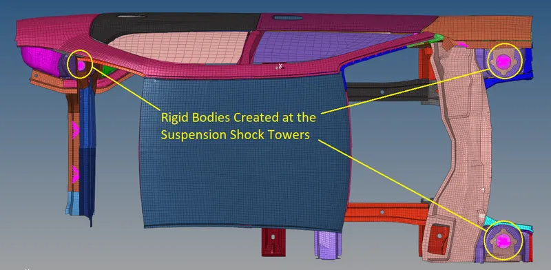
Now inorder to apply boundary condition to the suspension shock tower go to the BCS collector created, select the master node of RBODY as shown in figure below

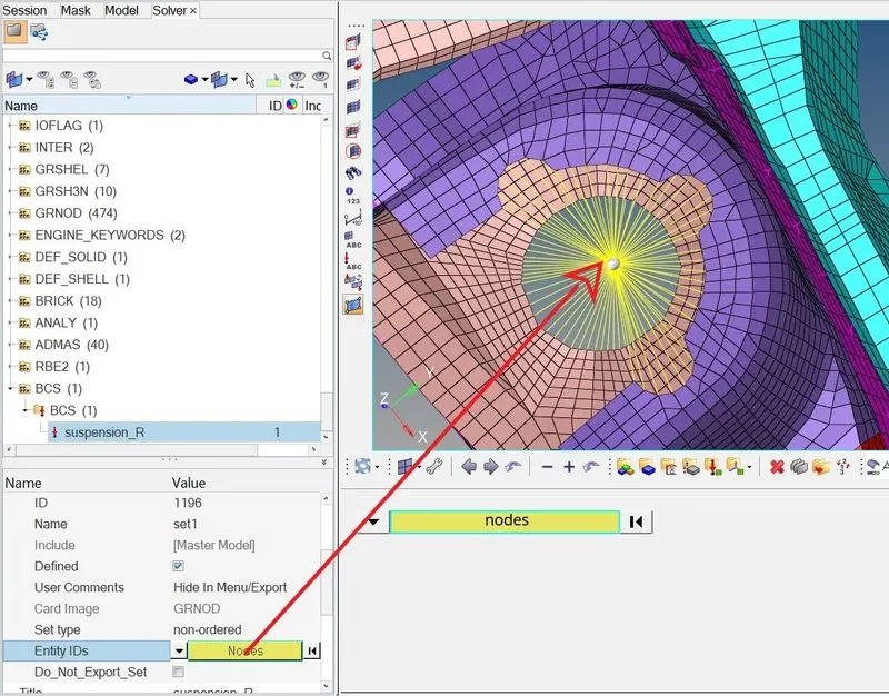
In order to keep the suspension shock tower nodes locked in Z direction, we need to check the DOF3 & DOF6 that will arrest both translational & rotational motions in Z direction.

Impactor Boundary Conditions

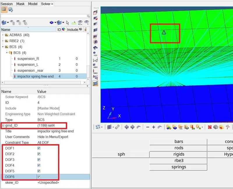
The impactor assembly contains a spring attached for stability. so we need to create a BCS collector to fix the free end of the spring.

as we can see in the figure, node at the free end of impactor spring is selected and checked all DOF in order to restrict motion in all direction.

Create a moving SKEW

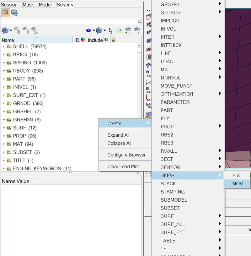
In order to define the direction normal to the impactor’s face. we need to create a moving skew, goto right-click on solver browser -> create -> skew -> MOV

select the origin node as master node of impactor, and axis we want to be normal and select the plane

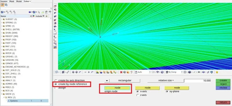
Create the boundary condition for the Master node of the impactor.

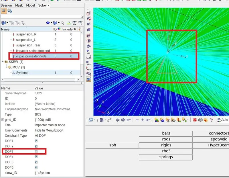
Create a BCS collector to guide the master node of the impactor rigid body, so that it is free to translate normal to the face of the impactor, but is fixed in all other DOFs.

As we can see in the figure below, BCS is applied at the master node of impactor and DOF3 is unchecked,so that it can move only in translational z-direction , all other movements in other directions are restricted.

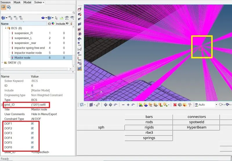
A boundary condition was applied on the master node of RBODY element on the right side of the car model, in order to rigidise the side.

Imposed Displacement

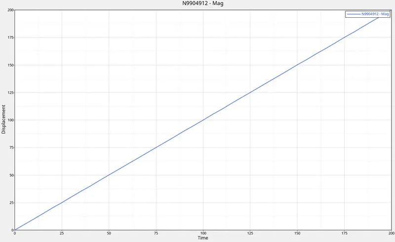
An imposed displacement has to be defined on the impactor master node such that the impactor moves from 0mm @ 0ms to 200mm @ 200ms. This helps in preventing any abrupt changes in the acceleration of the impactor. This can be defined as the function of the imposed displacement with XY coordinates at (0,0) and (200,200).

The function is created as follows:

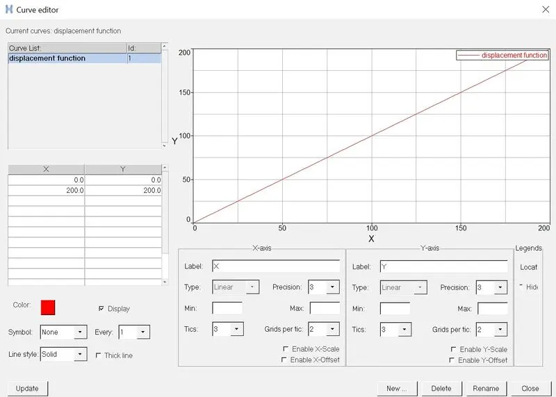
To create Imposed displacement boundary conditions, right-click on solver browser -> create -> Boundaryconditions -> IMPDISP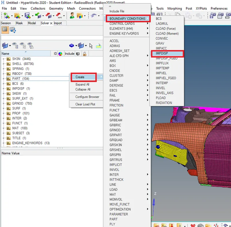

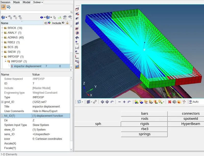
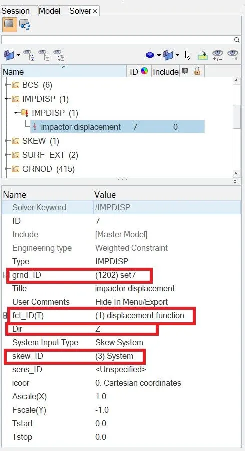
The imposed displacement is defined to the impactor master node and is defined with the displacement function and the Skew created before.

The direction is given as Z with respect to the skew. If the direction of application of the velocity is not in the downwards direction put the scale factor as -1 to adjust the direction.

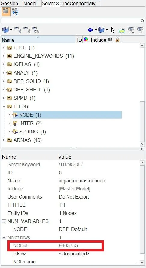
Creating Output block for Node

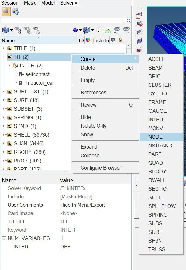
In order to find the displacement, we can create a TH (Time History ) file for the Master node of Impactor, go to

solver browser -> right-click on TH card -> create -> NODE, select the master node

Defining Control Cards

In order to create Control cards we can go to Analysis -> control cards option and select the required control cards.

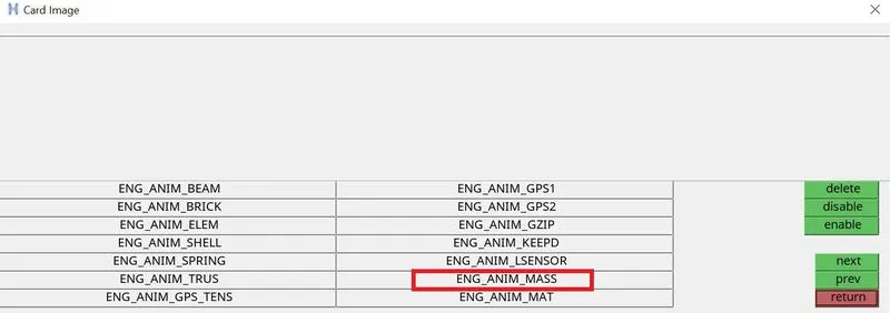
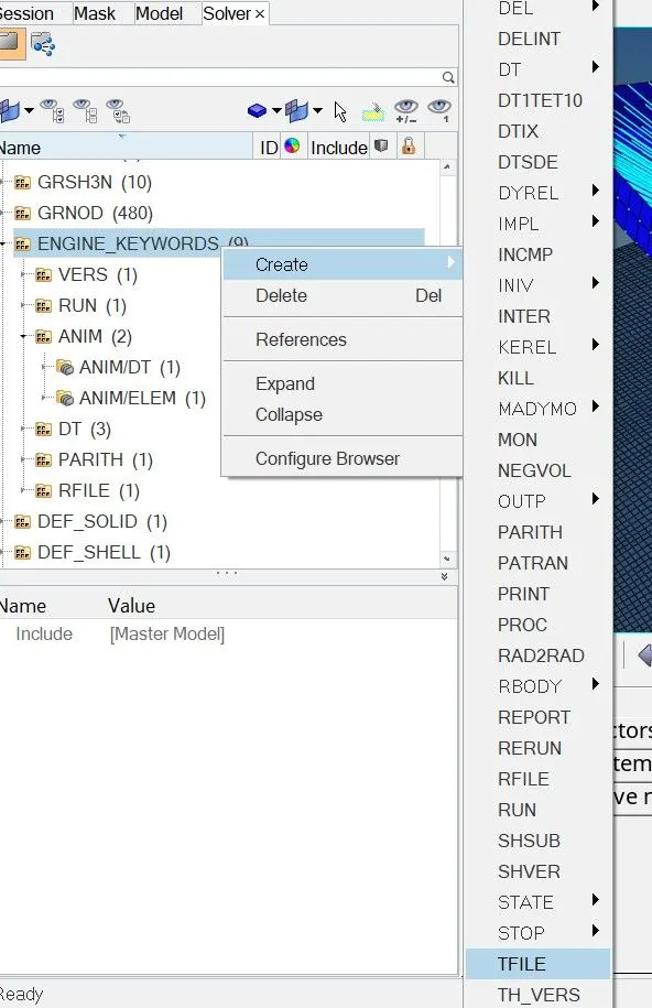
or we can go to solver browser -> Engine Keywords -> right click -> create as shown in figure below

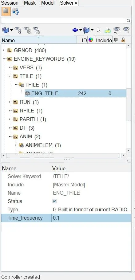
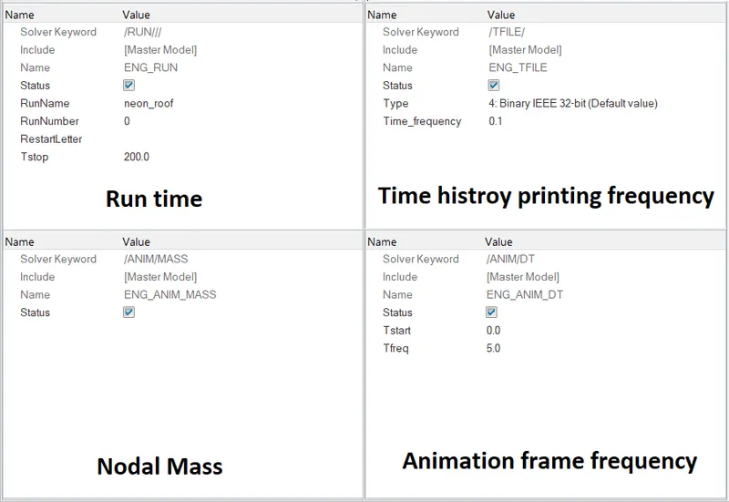
Required control cards created as shown in figure below

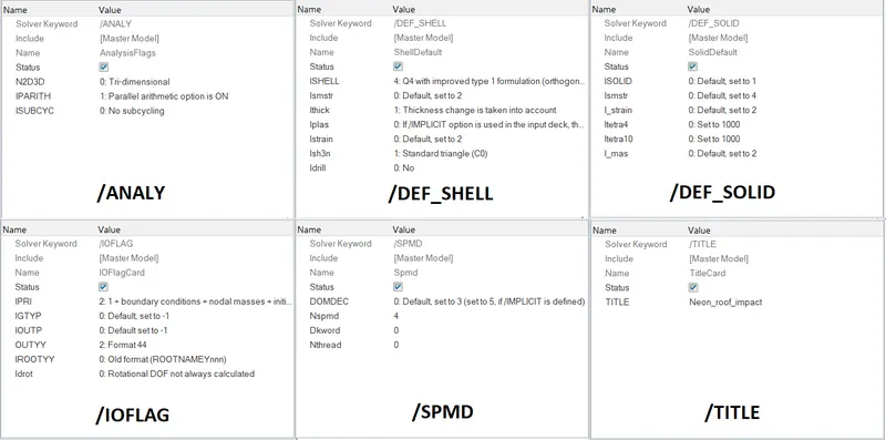
Defining Engine_Keywords File

The run time is set to 200 ms. The time history printing frequency is set to 0.1ms. The nodal mass animation is switched on. The animation frame frequency is set to 5ms.

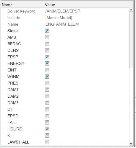
The Elemental Animation (/ANIM/ELEM ) is switched on for elemental energy, plastic strain, hourglass energy, von Mises stress.

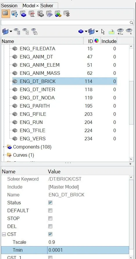
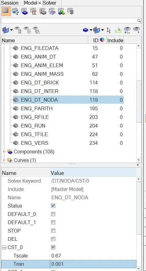
Inputting, Timestep for BRICK/INTER/NODA, got to Engine Cards

Check for connectivity in the Model

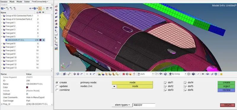
Before proceeding to run the simulation, we need to ensure the connectivity in the model. For that in HyperMesh, go to

Tools -> Find connectivity ->select all components in the car BIW -> check ,it shows many free parts in the model as shown in figure below

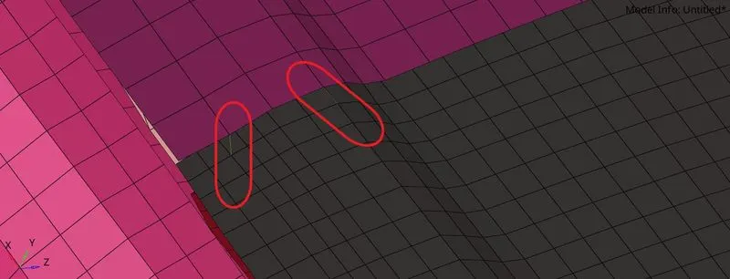
In order to keep connectivity between 2 parts we can create a Rigid connection between them, go to 1D -> Rigids ->Create

select nodes from each parts and create rigid connection between them, as shown in figure below.

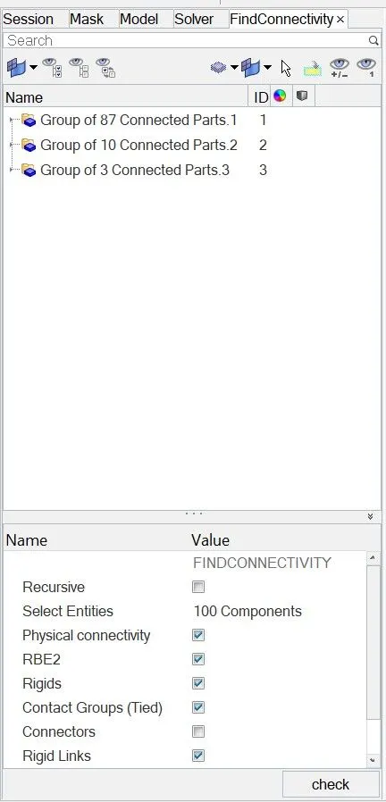
After connecting all free parts with Rigid connections, we check for connectivity again and found out no free parts exist in the model

Model Checker

As the final step before running the analysis model has to be checked for any errors and warnings,

we run the Model checker in Hypercrash, go to Quality > Model Checker > Run from the upper toolbar.

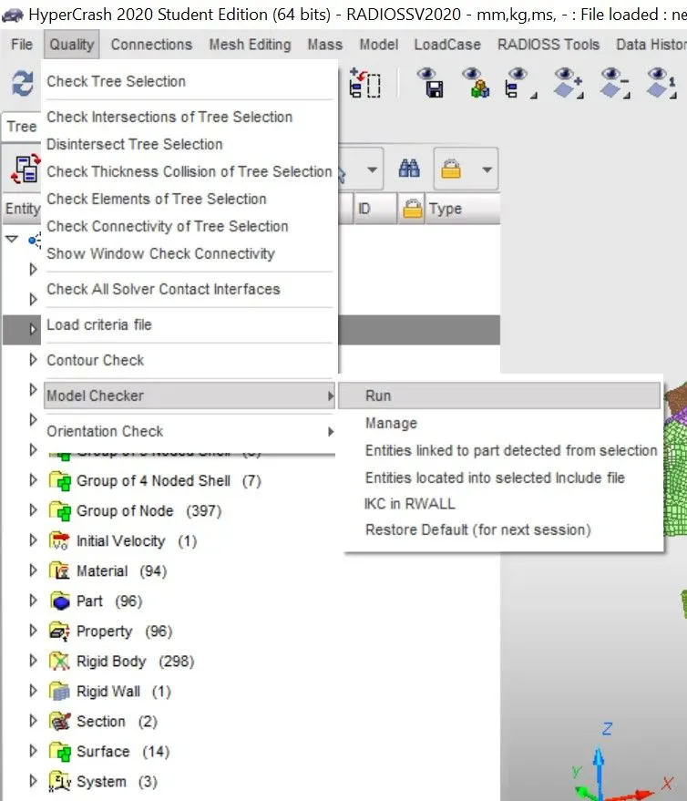
result is shown in figure below..there are a few errors present in the setup, so we need to debug the errors.

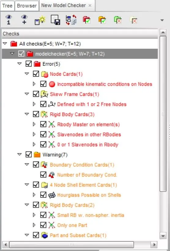
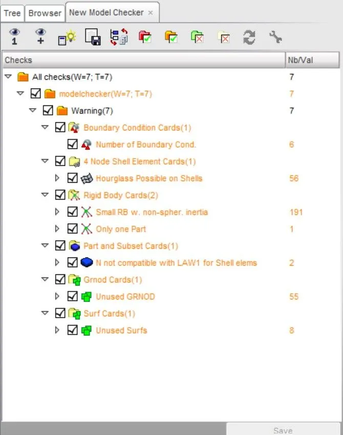
After debugging the errors we run the model checker again, and only some warning leftout, which can be avoidable

Run the Simulation

To run this simulation we have to use the Radioss command in the Analysis tab. Analysis -> RADIOSS

we can click 'save as' to save the file if it hasn't been saved yet. Care must be taken to include '_0000.rad' in the file name since it's the starter file.

After that, we can check the connectors option and input '-nt 4' in the options bar in order to use parallel arithmetic for using parallel tasking.

then click 'Radioss'. This starts the Radioss simulation.

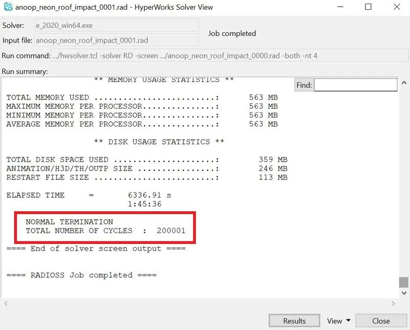
After the simulation is run, we can confirm that the simulation has run properly when we see a NORMAL TERMINATION at the end of the simulation ,as shown in fig below

ANALYSING THE OUTPUT FILE

The next step is to carry out energy error and mass error checks and this is done by analyzing the RADIOSS engine output file.

This can be accessed from the same directory as the starter and engine files and is denoted by the '.out' extension.

The file in question contains '_0001.out' and can be accessed using any text editor - such as Notepad.

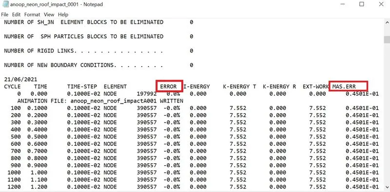
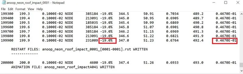
As we can see, the energy error is -19 %. It is slightly more than the acceptable range of -15 % to +5% error. this might be due to components breaking away from the model, since this a reduced car BIW, and some components of the model are not properly connected, there could be flying components that will lead to slightly more release of energy.

In addition to that, the mass error is 0.0467, which means that a negligible quantity of mass was added during the simulation, possibly for the sake of time step control/stabilization. It is a rather low amount so it's still acceptable.

SIMULATION ANIMATION

To view the simulation, we can switch to Hyperview through the client selector.

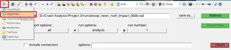
In Hyperview, we will need to import the .h3d variant of the file and hit Apply

Then the contour panel is opened, which appears as shown in fig below. In which the parameters to view the simulation are selected. Such as: result type in terms of Displacement, von misses stress etc. then selecting the components & apply.

Displacement contour plot

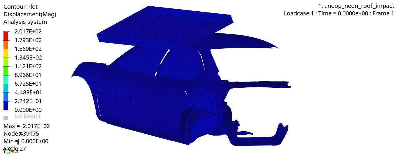
Maximum displacement occurred = 201.7 mm

Von Mises stress contour plot

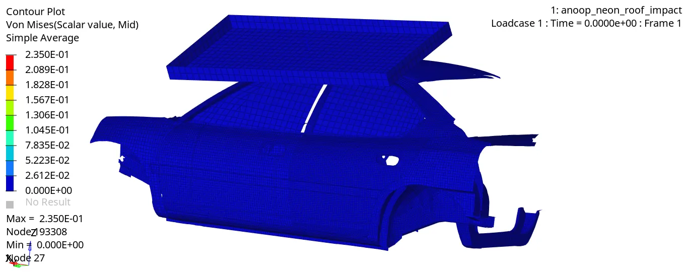
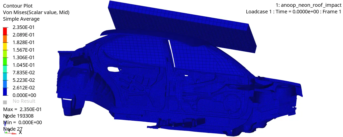
Von Mises stress is a value used to determine if a given material will yield or fracture. It is mostly used for ductile materials, such as metals. The von Mises yield criterion states that if the von Mises stress of a material under load is equal or greater than the yield limit of the same material under simple tension then the material will yield.

Maximum Von Mises stress = 0.235 Gpa

Impact versus Quasi Static Simulations

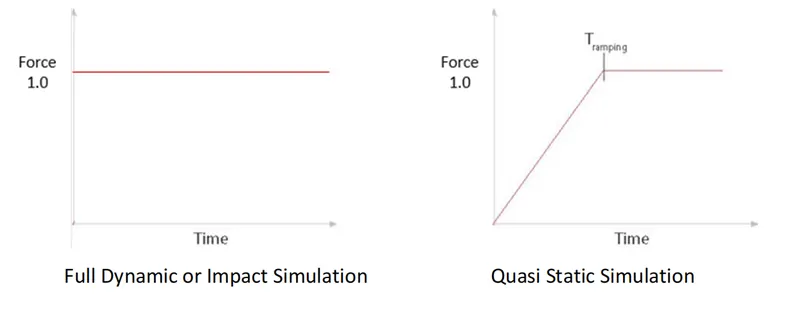
If the excitation frequency is less than one-third of the lowest natural frequency of the structure it can be considered a quasi-static loading where the inertial effect can be neglected. The term Quasi-Static is used to represent a slow dynamic process as opposed to a fast dynamic process. The distinction between these two is quite obvious when we see the load application in the following figure, a suddenly applied load (mathematically a heavy side or step input) will result in a displacement two times that of the static displacement of the system. The term Quasi-Static simulation is used when we use a dynamic code to produce a static result. It must be remembered that we will get a static or close to static result only if the ramp-up time is sufficiently large (i.e. the ramp-up slope is not too steep so as to get a close result as same as that as Full dynamic simulation).

Quasistatic simulation we have following options:

a. Increase the element length

b. Increase the density of the component, increasing the mass of component

c. Increase the rate of loading

d. Decrease elasticity moduli of the material

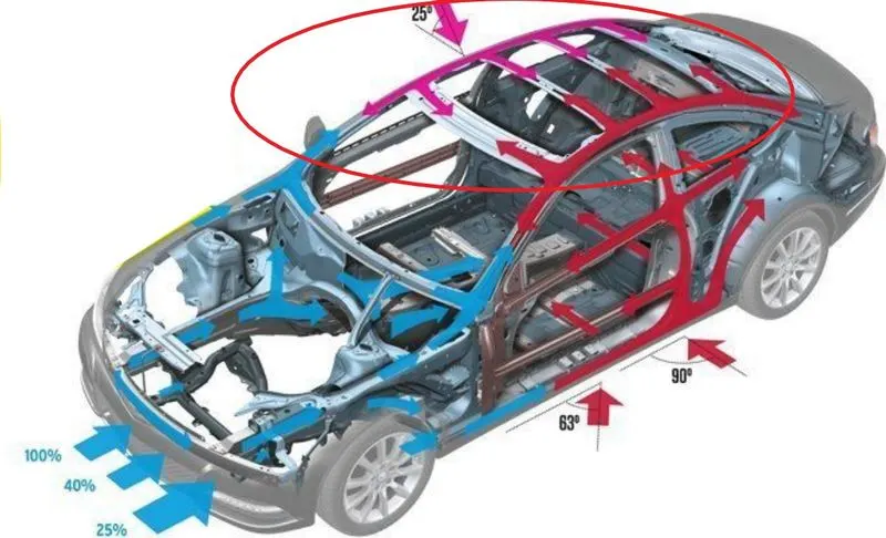
Load-carrying Path and Crash Process:

Generally, vehicles have a high relative velocity in crashes. For this reason

GENERATING OUTPUT PLOTS

After generating the simulation, we can then go ahead and generate the plots. Using the same client selector, we can switch to Hypergraph. In the Hypergraph client, we need to import time history file T01 file

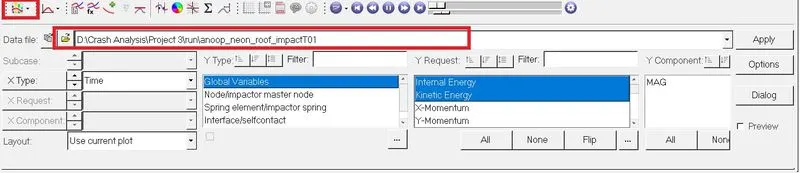
On importing, we can build the plots using different variables. We shall first look at general plots of energies and rigid wall forces generated in and by the entire BIW respectively.

GLOBAL VARIABLE GRAPHS: ENERGIES

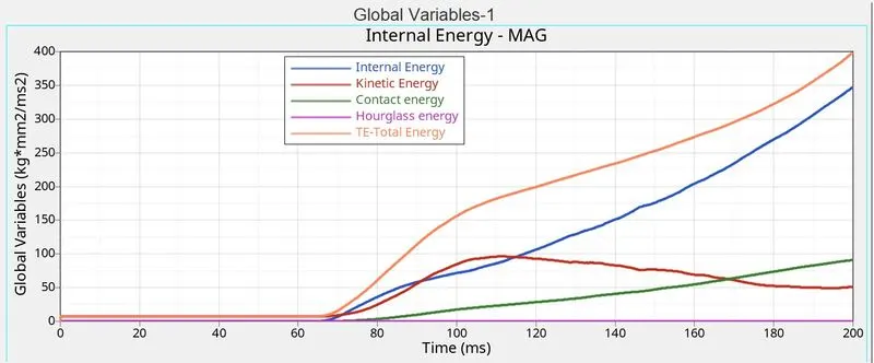
From the above Energy Plot we observed that,

For the first 70 ms there is no contact between BIW Component and Impactor. After 70 ms roof when the impactor hits the roof, Internal Energy starts to gain the energy of the system due to changes in its internal state of elements due to deformation and Maximum Internal Energy is 347.03 Kg*mm2/ms2 is generated.

Kinetic energy (KE) of an object is the energy that it possesses due to its motion. In the Simulation, the Vehicle is in rest condition, so there is no Kinetic energy will be generated. After 70 ms when the impactor hits the roof, KE starts to increase and reaches a maximum value of 96.4 Kg*mm2/ms2 at time t=111 ms will be created because of the motion produced on the components due to sudden impact on the car by the impactor. At the end of the simulation, then the KE starts to decrease.

We Know that Total Energy remains constant(no loss or generation of energy), Kinetic Energy decreases while Internal Energy Increases. But in this less Kinetic Energy and more Internal Energy is generated. So that Total Energy is 398.26 Kg*mm2/ms2 at t=200ms.

Contact energy is a type of energy that is formed when one element comes in contact with the other or neighboring elements. The opposing force created by this element forms the contact energy. In this case, contact energy increases after 80 ms, at this point the model starts deforming in such a way that penetration of nodes occurs. When certain regions of the model press on themselves, buckled elements are forced into contact.

From the above graph, we can see that the Hourglass energy is almost negligible since we have used Improved integrated element formulation (QEPH).

Force v/s Displacement plot

To plot Force vs Displacement curve, first we need to plot force vs time and displacement vs time, by taking both graphs we are cross plotting.

we have applied an imposed displacement of 200 mm to the impactor, so the Displacement vs time plot is as shown in figure below

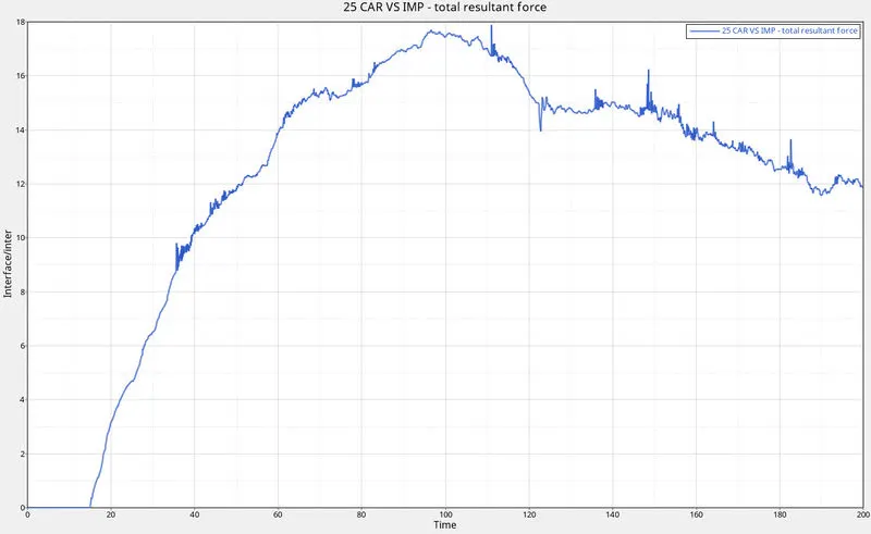
Force v/s time graph is obtained from the interface created between the Impactor and car BIW, as shown in figure below,

By cross plotting both the above 2 graphs, we have Displacement vs Force graph shown in the figure below

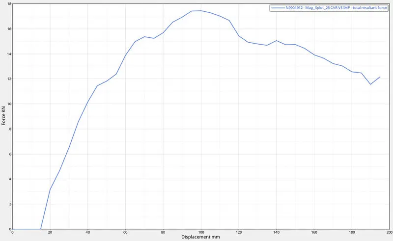
From the plot, we have Maximum force of 17.43 KN at 100 ms

Strength to weight ratio=(Resistive Force)/(Gross weight of the Vehicle)

47,000 N (= 3 * GVW) has been met.

Resistive Force = (Strength to weight ratio) *(Gross weight of the Vehicle)

Resistive Force = 3*9.81*174.05 = 5122.29N , this is the theoretical value.

Resistive force does Not exceed the 47000N, the Car is safe

From the graph

we have Resistive Force is 17.43KN = 17430 N

Gross weight of the Vehicle is 174.05*9.81 = 1,707.43 N ( Reduced car model weight = 174.05 kg)

Strength to weight ratio=Resistive Force/Gross weight of the Vehicle

Strength to weight ratio = 17430/1,707.43 = 10.2

Strength to weight ratio 10.2 because we taken only reduced car BIW weight as Gross weight

suppose if we consider full car model weight of 700 kg,

Strength to weight ratio = 17430/700*9.81 = 2.5 ,so it is Marginal

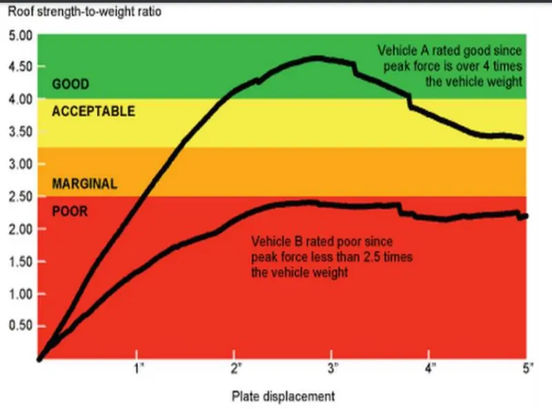
From the graph, it assigns a rating of Good(SWR greater than 4.0), Acceptable (SWR greater than 3.25 and up to 4.0),

Marginal (SWR greater than 2.5 and up to 3.25) or Poor (SWR less than 2.5).

For us, the model obtained the SWR of 2.5, so it is Marginal

Conclusion:

The overall objective of the work was to simulate roof crash analysis and validate the results of the simulations obtained from the Roof crash test. Simulation was performed using the Radioss solver.

The output is visualized using Hyperview and to determine the strength of the roof, cross plot is created in HyperGraph.

Due to the limited number of nodes in the student version some of the components of BIW, engine blocks, suspension system etc are removed, so results are not as in real condition.

It has been observed that Resistive force is Not exceeded value 47000N, the Car is safe

It has been observed that considering the total car weight 700 Kg the Strength to weight ratio is Marginal.