Week 4.1 - Genetic Algorithm

clear all
close all
clc

%% Determining minima values for the stalactites

% Creating an array of 1D
xi = linspace(0,1,200);
yi = linspace(0,1,150);

% Creating a mesh of x and y
[X,Y] = meshgrid(xi,yi);

% Creating a dummy matrix of length(yi)*length(xi)
f =nan(size([length(yi) length(xi)]));

% Specifying co-ordinates within the grid and getting values at those
% points

for i = 1:length(yi)
    for j=1:length(xi)
    
    % Segregating the x and y co-ordinates into a 2 element matrix       
    input_vector(1) = X(i,j);
    input_vector(2) = Y(i,j);
    
    % Calculating the minima values of stalactites  
    f(i,j) = stalagmite(input_vector);
     
    end
end

%% Study_1 - Statistical behaviour, Unbounded, default population size

num_cases = 50;
f_output_study1 = nan(1,num_cases);
x_output_study1 = nan(1,num_cases);
y_output_study1 = nan(1,num_cases);

tic
for i=1:num_cases
    
    [inputs,f_output_study1(i)] = ga(@stalagmite,2);

% As programmed, ga calculates the minima of any function
% nvars = 2 happens to be the number of input variables, in this case, x&y.
% inputs are the coordinates for minima.
% in the above syntax, ga is calculating the lowest points of stalactites
% f_output_study1 values are magnitude of minima corresponding to the resp coordinates.

    x_output_study1(i) = inputs(1);
    y_output_study1(i) = inputs(2);   
end
study_1_time = toc;

% Plotting

figure(1)
subplot(2,1,1)
% Using -f, to convert stalactites back into stalagmites!
surf(xi,yi,-f)
zlim([-0.2 1.5])
shading interp
hold on
plot3(x_output_study1,y_output_study1,-f_output_study1,'marker','o','markersize',5,'markerfacecolor','r')
% Again a -f to get stalagmites from stalactites
hold off
xlabel('X axis')
ylabel('Y axis')
zlabel('Stalagmite function value - f')
title('Unbounded inputs for stalagmite function')
subplot(2,1,2)
plot(-f_output_study1)
xlabel('Iterations')
ylabel('function maximum')

%% study_2 - Statistical behavious, with lower and upper bounds respectively

f_output_study2 = nan(1,60);
x_output_study2 = nan(1,60);
y_output_study2 = nan(1,60);


tic
for i = 1:60
    [inputs,f_output_study2(i)] = ga(@stalagmite,2,[],[],[],[],[0;0],[0.6;0.6]);
    x_output_study2(i) = inputs(1);
    y_output_study2(i) = inputs(2);
    
end
study_2_time = toc;

% Plotting

figure(2)
subplot(2,1,1)
surfc(X,Y,-f)
shading interp
hold on
plot3(x_output_study2,y_output_study2,-f_output_study2,'marker','o','markersize',5,'markerfacecolor','b');
xlabel('X axis')
ylabel('Y axis')
title('Bounded Inputs with lower and upper bounds')
subplot(2,1,2)
plot(-f_output_study2)
xlabel('Iterations')
ylabel('function maximum')

%% Study 3 - Increasing ga iterations

f_output_study3 = nan(1,num_cases);
x_output_study3 = nan(1,num_cases);
y_output_study3 = nan(1,num_cases);

options = optimoptions('ga','PopulationSize',300);
nVars = 2;
tic
for i = 1:num_cases
    [inputs,f_output_study3(i)] = ga(@stalagmite,nVars,[],[],[],[],[0;0],[0.6;0.6],[],[],options);
    x_output_study3(i) = inputs(1);
    y_output_study3(i) = inputs(2);
    
end
study_3_time = toc;

% Plotting

figure(3)
subplot(2,1,1)
surfc(X,Y,-f)
shading interp
hold on
plot3(x_output_study3,y_output_study3,-f_output_study3,'marker','o','markersize',6,'markerfacecolor','b');
xlabel('X axis')
ylabel('Y axis')
title('Bounded Inputs with increased population size')
subplot(2,1,2)
%semilogy(-f_opt)
plot(-f_output_study3)
xlabel('Iterations')
ylabel('function maximum')

1. Attaching Error and output images.

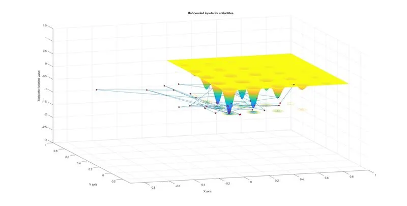
• Unbounded inputs for stalactites

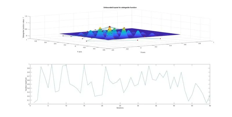
• Unbounded inputs for stalagmites

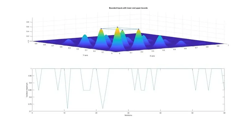
• Bounded Inputs with lower and upper bounds

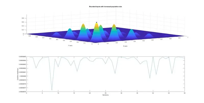
• Bounded Inputs with increased population size

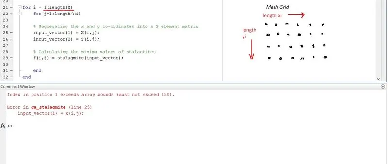
• Error-1, the details of which have been elucidated in the report attached as an individual word file.

Important Points

• Upon observing all the images, particularly the 2nd graph of each plot, we see the tolerance keeps on reducing. Thus we conclude that bounding the graph and increasing the population makes ga more optimized. Bounding is done based on users discretion and experience.
• Please be noted that the 3rd plot is having different number of iterations, 60, for "playing around with programming skills" of the user.
• The report is written in a word file, which is attached individually.