Week 8 - Simulating Cyclone separator with Discrete Phase Modelling

SIMULATING CYCLONE SEPARATOR

Aim:

To perform an analysis on cyclone separator and calculate the separation efficiency and pressure drop.

Objective:

To write a few words about any four empirical models used to calculate cyclone separator efficiency.

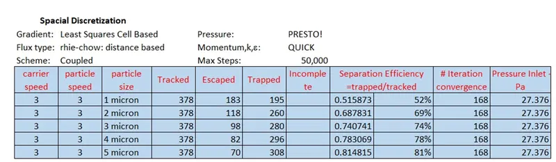
To perform an analysis on a given cyclone separator model by varying particle diameter from 1 to 5 microns and calculate separation efficiency in each case. Discuss the results. Use particle and flow velocity as 3 m/s

To perform an analysis on a given cyclone separator model by varying particle velocity from 1 to 5 m/sec and calculate separation efficiency and pressure drop in each case. Discuss the results.

{Use particle diameter size as 5 microns for all cases & keep flow velocity same as particle velocity}

Brief theory of cyclone separator

Cyclone separators are basically separation devices that use principle of inertia to remove particulate matter from flue gases.

These are usually designed to remove particle matter greater than 10 microns, but some can segregate for as low as 2.5 microns.

These are usually used in air pollution cleaning plant and work as pre-cleaners as they remove larger particles off the polluted air and send in the gases for further refinement.

A continuous feed of dirty flue air is fed into a chamber of cyclone separator, the insides then create a spiral vortex, similar to a tornado. Lighter particles, having lesser inertia, get influenced by vortex and flow up through an outlet.

Heavier particles having greater inertia, hit the inner walls of the separator and fall off to the bottom of the equipment wherein they are collected in a bottom pan.

In the literatures, there are two typical ways for improving cyclone performance. The first modification is about cyclone's is about the flow characteristics like velocity inlet condition or temperature. For example inlet gas velocity is an effective parameter on the cyclone performance and increases pressure drop

The second modification is about the flow characteristics like velocity inlet condition or temperature. For example, inlet gas velocity is an effective parameter on the cyclone performance and increases pressure drop.

Empirical models used to calculate the cyclone separator efficiency.

• Lapple
• Koch and Licht
• Li and Wang, and
• Iozia and Leith

Iozia and Leith

Iozia and Leith logistic model is a modified version of Barth Model, which was developed based on force balance. The model assumes that a particle carried by the vortex endures the influence of two forces: a centrifugal force, Z and a flow resistance, W.

Li and Wang

The Li and Wang model includes particle bounce or re-entrainment and turbulent diffusion at the cyclone wall. A two-dimensional analytical expression of particle distribution in the cyclone is obtained. Li and Wang model was developed based on the following assumptions:

• The radial particle velocity and the radial concentration profile are not constant for uncollected particles within the cyclone.
• The tangential velocity is related to the radius of cyclone.

Koch and Licht

Koch and Licht collection theory recognized the inherently turbulent nature of cyclones and the distribution of gas residence times within the cyclone.

Koch and Licht collection theory recognized the inherently turbulent nature of cyclones and the distribution of gas residence times within the cyclone.

Lapple:

Lapple model was developed based on force balance with-out considering the flow resistance. Lapple assumed that a particle entering the cyclone is evenly distributed across the inlet opening. The particle that travels from inlet half width to the wall in the cyclone is collected with 50% efficiency.

Before starting with simulation steps, a brief understanding of “behind the scenes”, the theory!

An attempt to decode, analyse and comprehend the Viscous Model dialog box

Selecting a “Model”:

Here, we select a “k-epsilon (2 eqn)” model – this is, as the name says, a 2-equation model, the 2 equations being a transport equation for turbulent kinetic energy, k, and transport equation for turbulent dissipation rate `ϵ`.

• Understanding the `k-ϵ` model

The transport equation for the mean flow velocity is solved using RANS equation.

RANS – Reynolds averaged Navier Stokes equation contains a Reynolds Stress term as shown below.

Reynolds stress is product of two fluctuating velocity components averaged over and divergence taken of that term `∇.(ρU^' U^' )`

`(∂(ρU))/(∂t)+∇ .(ρUU)= -∇p+∇.[μ(∇U+(∇U)^T )]+ρg-∇(2/3 μ(∇.U))-(∇.((ρU^' U^' ) ) ) (1)`

In order to solve for mean velocity U, we need to close the equation by solving Reynolds stress term.

Reynolds stress term is modelled by using Boussinesq hypothesis, the details of which, we shall not delve into in this challenge.

Reynolds stress is related to mean velocity gradients by turbulent viscosity or dynamic eddy viscosity `μ_t`.

`μ_t=C_μ (ρk^2)/ϵ (2)`

In order to calculate this “dynamic eddy viscosity, `μ_t` ” we need to solve a transport equation for two turbulent quantities – the turbulent kinetic energy, k and turbulent dissipation `ϵ.`

Transport equation for turbulent kinetic energy, k is the same for all the `k-ϵ` models (Standard, RNG and Realizable)

The variations seen are in solution to the transport equation for `ϵ`.

This leads us to understand, briefly, some more about the RNG `k-ϵ` model.

Selecting a “k-epsilon Model”:

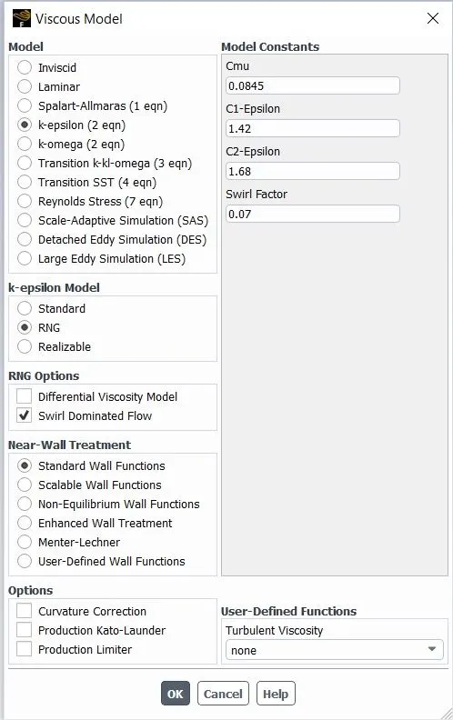
Here we select the RNG variant of k-epsilon model.

• Understanding RNG `k-ϵ` model

The RNG model was developed using Re-Normalisation Group (RNG) methods by Yakhot et al to renormalise the Navier-Stokes equations, to account for the effects of smaller scales of motion.

In the standard k-epsilon model the eddy viscosity is determined from a single turbulence length scale, so the calculated turbulent diffusion is that which occurs only at the specified scale, whereas in reality all scales of motion will contribute to the turbulent diffusion.

The RNG approach, which is a mathematical technique that can be used to derive a turbulence model similar to the k-epsilon, results in a modified form of the epsilon equation which attempts to account for the different scales of motion through changes to the production (generation, G_k) term.

Why RNG `k-ϵ` model?

• The RNG model has an additional term in its `ϵ` equation that improves the accuracy for rapidly strained flows, example in converging part of a nozzle.
• The effect of swirl on turbulence is included in the RNG model, enhancing accuracy for swirling flows – This is the reason we choose this solver for our current simulation.
• The RNG model is more responsive to the effects of rapid strain and streamline curvature than the standard `k-ϵ` model.

Selecting “RNG Options”:

Here we have two options which can be selected, these are

1. Differential Viscosity Model.
2. Swirl Dominated Flow.

• Differential Viscosity Model

The formula for calculating dynamic eddy viscosity, `μ_t` , has two forms, one of which is chosen depending on the option we select.

One of the forms is a differential form under RNG class of `k-ϵ` model, this formula accounts for low Reynolds number.

The other form, is the formula as stated above. This is used for high Reynolds number flows.

As our challenge does not include a low Reynolds flow, we shall be going with the latter.

Differential viscosity model is selected for low Re flows.

For this reason, we shall not be selecting Differential Viscosity Model flow.

• Swirl Dominated Flow

Turbulence, in general, is affected by rotation or swirl in the mean flow.

The RNG model in Ansys Fluent provides an option to account for the effects of swirl or rotation by modifying the turbulent viscosity appropriately.

The modification takes the following functional form –

`μ_t=μ_(t0) f(α_s,Ω,k/ε) (3)`

Here `μ_(t0)` is the value of turbulent viscosity calculated without the swirl modification as stated in the discussion above.

Omega, `Ω`, is a characteristic swirl number evaluated within Ansys Fluent

And `α_s` is a swirl constant that assumes different values depending on whether the flow is swirl-dominated or only mildly swirling. This swirl modification always takes effect for axisymmetric, swirling flows and three-dimensional flows when the RNG model is selected. For mildly swirling flows (the default in Ansys Fluent), `α_s` is set to 0.07. For strongly swirling flows, however, a higher value of `α_s` can be used.

We check the swirl dominated flow as our simulation is one.

Near Wall Treatment:

Here we shall go ahead with the standard wall functions.

Wall functions:

There are two ways for modelling near wall region.

In one approach, the viscosity affected inner region (viscous sublayer and buffer layer) is not resolved. This is called the “wall functions” approach. The second approach is to mesh all the way to the wall, including the viscous sublayer, one could call this as near-wall modelling.

“Wall functions” provided by Ansys are Standard, Scalable, Non-Equilibrium and User-Defined Wall Functions.

Wall functions are a set of semi-empirical formulas and functions that in effect “bridge” or “link” the solution variables at the near-wall cells and the corresponding quantities on the wall.

The standard wall functions in Ansys Fluent are based on the work of “Launder and Spalding” and have been most widely used in industrial flows. They are provided as a default option in Ansys Fluent.

Material: Anthracite-volatiles (an_vol), Fluid

Anthracite is a high-rank shiny black, hard and brittle coal. It is low in volatile matter and this makes it difficult to burn in rotary kilns. They have low-moisture content. They have low content of sulphur and volatiles. These volatile particulate matters, having varying sizes, can be trapped in a cyclone separator.

Modelling Discrete Phase

This modelling shall be based on the Lagrangian concepts.

In addition to solving transport equations for the continuous phase, Ansys Fluent also allows us to simulate a discrete second phase in a Lagrangian frame of reference. This second phase consists of spherical particles (anthracite volatiles in our simulation) dispersed in the continuous phase (air in this simulation).

Ansys Fluent computes the trajectories of these discrete phase entities, as well as heat and mass

transfer to/from them.

The coupling between the phases and its impact on both the discrete phase trajectories and the continuous phase flow can be included.

These calculations include the discrete phase inertia, hydrodynamic drag, and the force of gravity, for both steady and unsteady flows (steady state flow chosen in our simulation).

Interaction with Continuous phase:

Enabling “Interaction with Continuous phase” will lead to coupled DPM simulation.

For a better understanding of ensuing paras, let it be noted that fluid flow (Carrier phase) is air and particle flow is anthracite.

When the fluid changes the particles, there will be corresponding effects on the fluid as well. For example, when drag force acts on a particle, the exchange of momentum can change the fluid flow.

In a Coupled DPM simulation, the effects of the particles are used to influence the flow solution.

These effects are transmitted to the flow as DPM Sources. Thus, updating DPM sources every flow iteration shall will ensure correct carrier phase flow simulation.

DPM Dialog Box:

• Particle Treatment

Steady Treatment of Particles –

The Discrete Phase Model uses a Lagrangian approach to derive the equations, which are solved transiently.

Transient numerical procedures in the Discrete Phase Model can be applied to resolve steady flow simulations as well as transient flows, with our simulation having a steady flow solution.

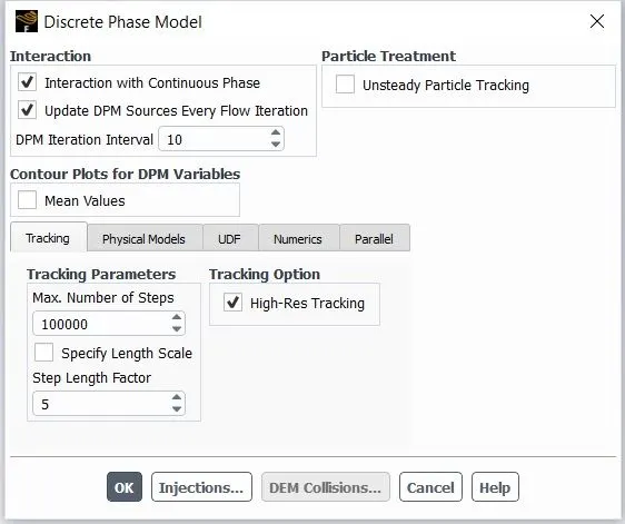
Tracking Parameters:

Max. Number of Steps –

This is the maximum number of time steps used to compute a single particle trajectory via integration of the Equation given below

`m_p (d((u_p ) ⃗ ))/dt=m_p (u ⃗- (u_p ) ⃗ )/τ_r +m_p (g ⃗(ρ_p-ρ) )/ρ_p +(F ) ⃗ (4)`

Where `m_p` is mass of the particle, `u ⃗` is fluid phase velocity, `(u_p ) ⃗` is particle velocity, `ρ` is fluid density, `ρ_p` is density of the particle, `F ⃗` is an additional force.

First term on RHS of equation is the drag force.

When maximum number of time steps are exceeded, particle trajectory calculations are terminated and trajectory fate is reported as “incomplete”.

The limit on the number of integration time steps eliminates the possibility of a particle being caught in a recirculating region of the continuous phase flow field and being tracked infinitely.

Step Length Factor –

This factor controls the time step size used to integrate the equations of motion for the particle.

The integration time step size is computed by Ansys Fluent based on a characteristic time that is related to an estimate of the time required for the particle to traverse the current continuous phase control volume. If this estimated transit time is defined as `∆t^*` , Ansys Fluent chooses a time step size, `∆t` as

`∆t=(∆t^*)/λ (5)`

`λ` is the step length factor. Increasing this value will reduce the time step size.

This is roughly equivalent to the number of time steps required to traverse the current continuous phase control volume. Default value for this is 5.

As shown in the diagram below, When Accuracy Control is enabled in the “Numerics” tab, the settings for Step Length Factor and Length Scale will be used only to estimate the time step size of the first integration step.

In all subsequent integration steps, the particle integration time step size is adapted to achieve the tolerance specified.

Accuracy control enables the solution of equations of motion within a specified tolerance.

This is done by computing error of integration step and reducing that step if error is too large. Contrarily, if error is within tolerance, then integration step is increased in subsequent steps.

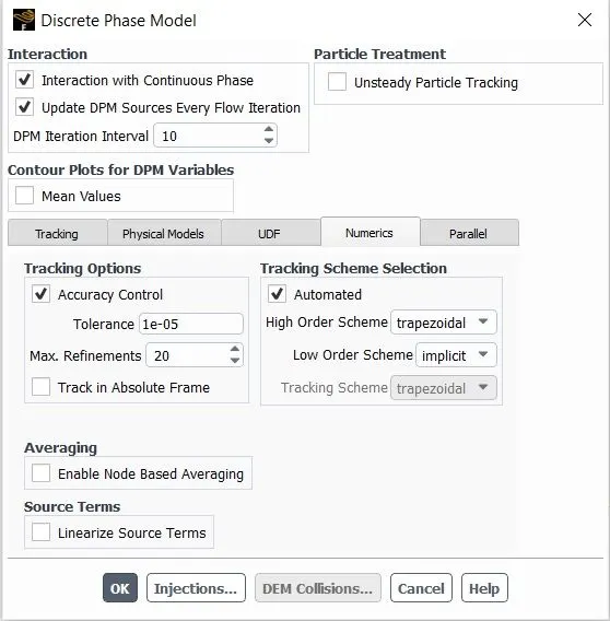
High-Res Tracking –

If High-Res Tracking is not enabled, particles are tracked through the computational cells directly.

Flow variables that appear in particle equations either use cell-centre values or a truncated Taylor series approximation for interpolation to the particle position.

When the High-Res Tracking option is enabled in the Tracking Option group box, the computational cells are decomposed into tetrahedrons (subtets) and the particles tracked through the subtets. This option provides a more robust tracking algorithm and improved variable interpolation.

Particle Type –

An inert particle is a discrete phase element (particle, droplet, or bubble) that obeys the force balance.

Discrete Phase Boundary Condition Types:

Sets the way that the discrete phase behaves with respect to the boundary.

Reflect: Walls

The particle rebounds off the boundary with a change in its momentum as defined by the coefficient of restitution (for non-rotating particles).

• Coefficients of Restitution:

A normal or tangential coefficient of restitution equal to 1.0 implies that the particle retains all of its normal or tangential momentum after the rebound (an elastic collision). A normal or tangential coefficient of restitution equal to 0.0 implies that the particle retains none of its normal or tangential momentum after the rebound.

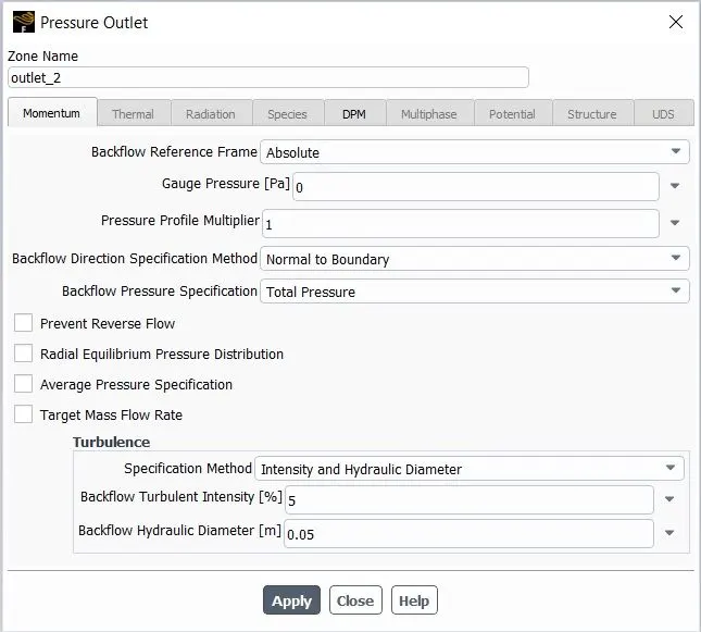
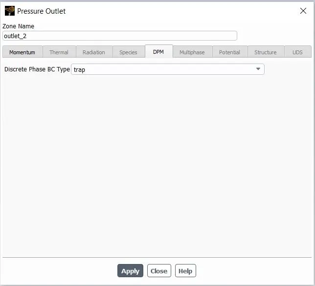
Trap: Outlet-2

Terminates the trajectory calculations and records the fate of the particle as "trapped". In the case of evaporating droplets, their entire mass instantaneously passes into the vapor phase and enters the cell adjacent to the boundary.

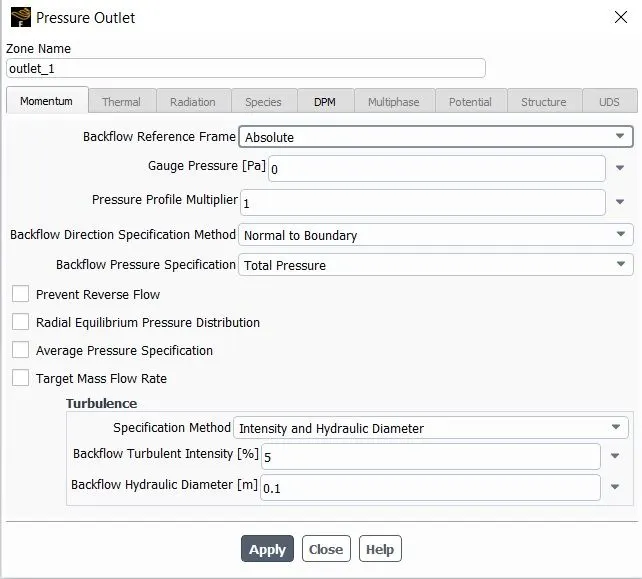
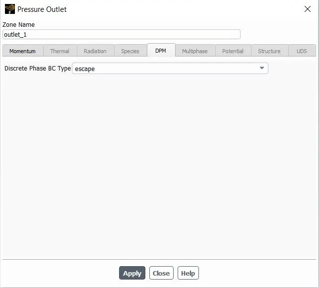
Escape: Outlet-1

Reports the particle as having "escaped" when it encounters the boundary. Trajectory calculations are terminated.

The reflect type is assumed at wall, symmetry, and axis boundaries, with both coefficients of

restitution equal to 1.0

The escape type is assumed at all flow boundaries (pressure and velocity inlets, pressure outlets,

and so on)

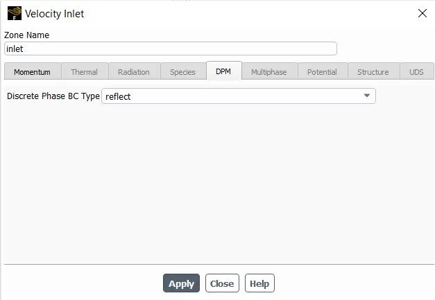
Reflect: Inlet

We can either select Reflect or Escape as an option for Inlet.

We select “Reflect” option for Inlet.

Solver Selection:

As our flow is low-speed and incompressible in nature, we shall select pressure-based solver.

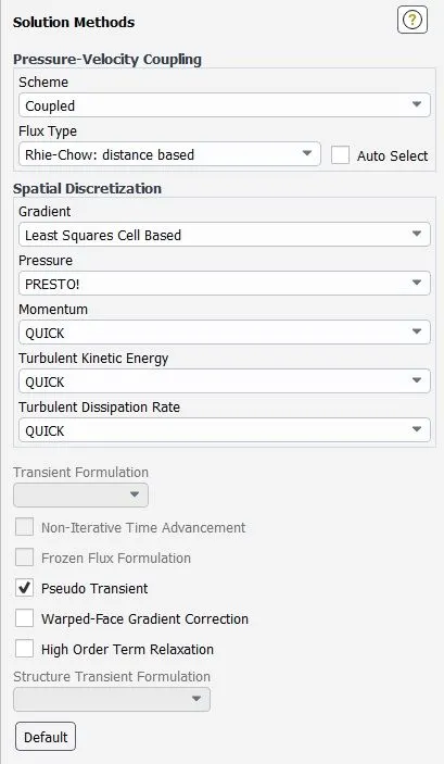
Solution Methods:

Why Coupled?

In general, segregated methods (SIMPLE, PISO etc) are faster per iteration, while the coupled algorithm usually requires fewer iterations to converge. For this reason, the coupled solver is usually recommended for steady state simulations.

Why PRESTO?

For pressure interpolation schemes, we use the “PRESTO” scheme – For high-speed rotating flows, and flows in strongly curved domains, the PRESTO! scheme is recommended.

A least square cell-based gradient is selected.

Why QUICK?

A QUICK Spacial Discretization Scheme is used for Momentum, turbulent kinetic Energy and Turbulent dissipation rate.

As per ANSYS Documentation, the QUICK and third-order MUSCL discretization schemes may provide better accuracy than the second-order scheme for rotating or swirling flows. The QUICK scheme is applicable to quadrilateral or hexahedral meshes.

In case of hybrid Meshes, were we have a combination of hexahedral and other forms of meshes, QUICK scheme shall be applied to hex cells and second order upwind scheme shall be applied to the rest of the cells.

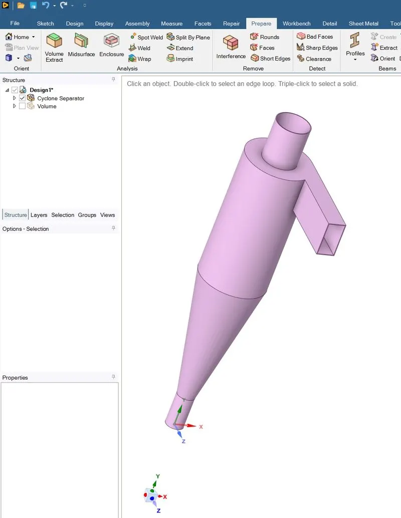
Geometry setup:

• Choose Fluid flow (fluent) module.
• Select geometry edit
• Import step file into SpaceClaim.
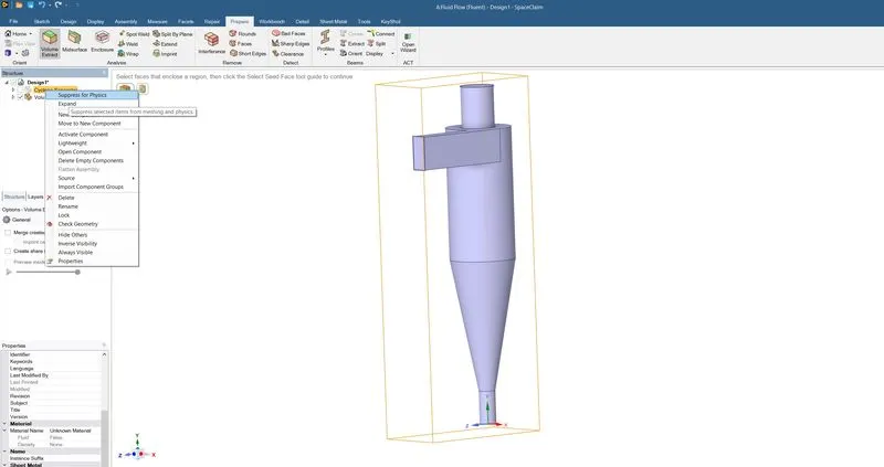
• Choose extract fluid volume.
• Hide solid body and suppress it for physics.

Mesh Setup:

• Main element size: 5 mm
• Method: Cartesian

1. Generate mesh and provide named selection to inlet, outlet top and outlet bottom.
2. Refine the mesh by reducing element size from default value of 55 mm as selected by Ansys to this specific model.
3. Verify the number of elements as it should not cross half a million cells as that is a restricting factor for student version.
4. The mesh cells generated are hex dominant in shape.

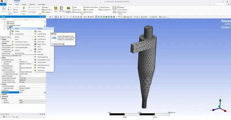
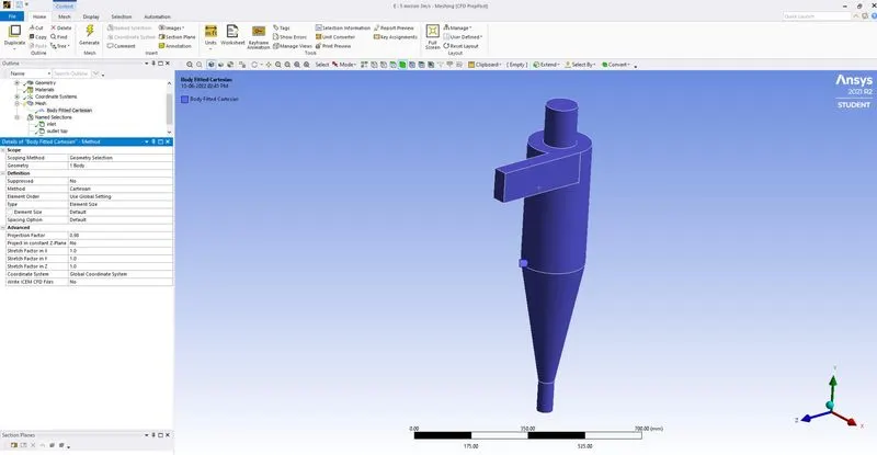
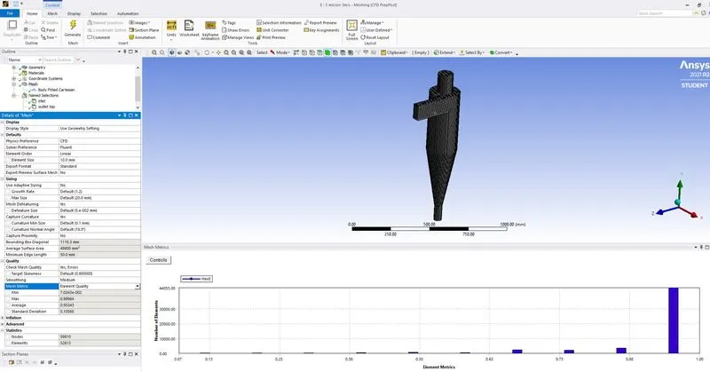
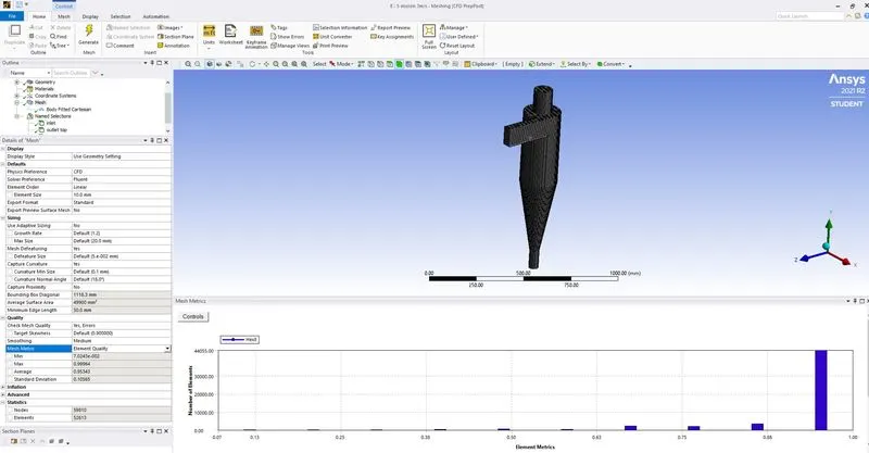
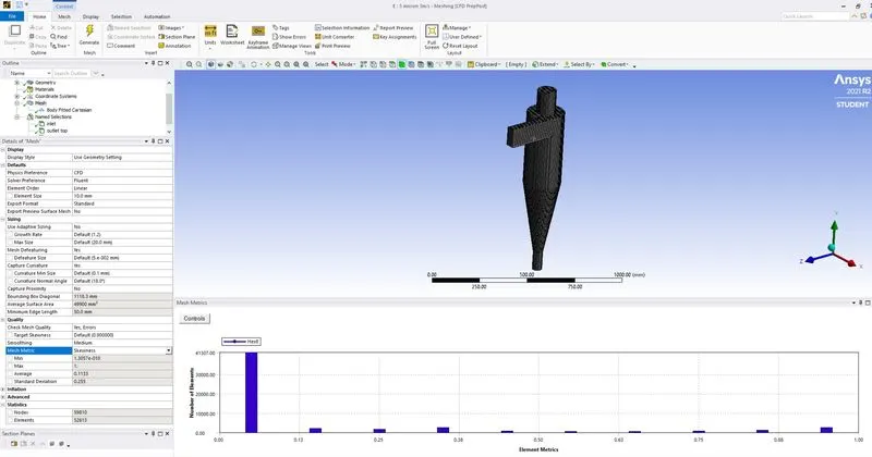
The element size taken is 5 mm and not 10 mm as the image shows. The total cells cross a value of 400,000. Total cells on inlet face are about 378. Mesh is structured as well.

Solver:

Start FLUENT.

• General
• Under setup tab in left column, click on General and select the following:
• Pressure-based under solver
• Absolute for Velocity Formulation
• Steady time
• Gravity in y axis as negative 9.81 meter per square second.

• Models
• Open Viscous model and select the following
• K-Epsilon (2 eqn), RNG, Swirl Dominated Flow, Standard wall Treatment.

• Open Discrete phase and check interaction with Continuous Phase.

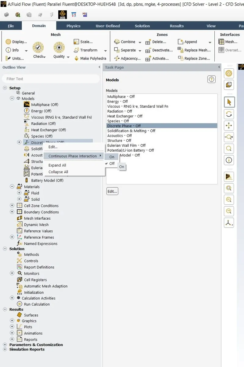
• Set DPM Sources interval to 10.
• Keep max. number od steps and step length factor as default of 100,000 and 5 respectively.
• Check Hi Res Tracking
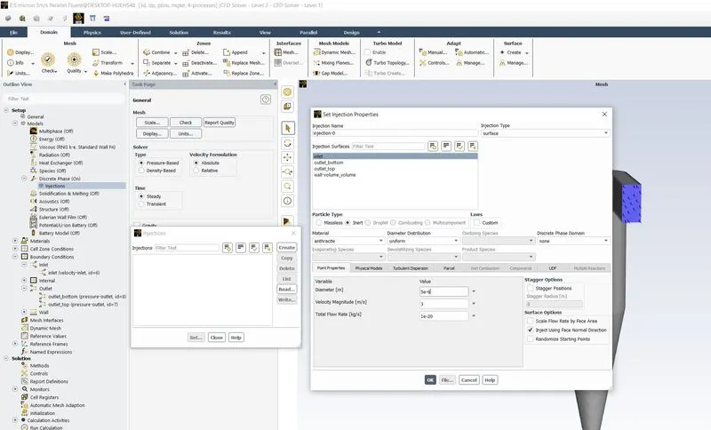
• Select injections at the bottom, an Injections tab is opened. Click on Create.
• Set Injection Properties tab opens. Give a user defined name under the Injection Name option.
• Under Injection Surfaces, select Input and surface type under Injection Type.
• Select Inert under Particle type.
• Diameter distribution is kept as default to uniform.
• Under point properties tab, give a velocity in x direction field as this is not with respect to the global coordinates but rather with respect to the local coordinates of the inlet.
• An alternative to the same is to check the Inject Using Face Normal Direction option in the right column and give an absolute value for the velocity of the incoming discrete particles as required.
• It is to be noted that this setting is for the particles that shall be in the flow, it is also called as the secondary phase or discrete particle phase.
• Now select a diameter as required in the simulation.
• Diameter selected is in microns. Varies for 1 to 5 microns.
• Keep the total flow rate as default to 1e-20 kg per second.

Material:

Select anthracite as the particle for simulation purposes, this step is already taken care of from previous step.

Cell Zone Conditions:

Under cell zone conditions, ensure air is selected in interior cells.

Air is the carrier phase.

Boundary Conditions:

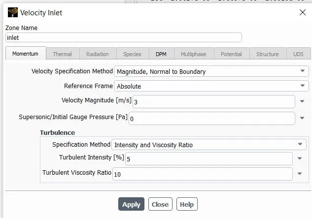
Under inlet boundary condition, set the velocity of air to a value as per cases selected.

Under outlet boundary conditions, ensure pressure-based outlet is selected.

Results for a particle size of 5 micron and varying velocities from 1 to 5 meter per second for both carrier phase and carrier are given below:

5 micron 1 meter per second case

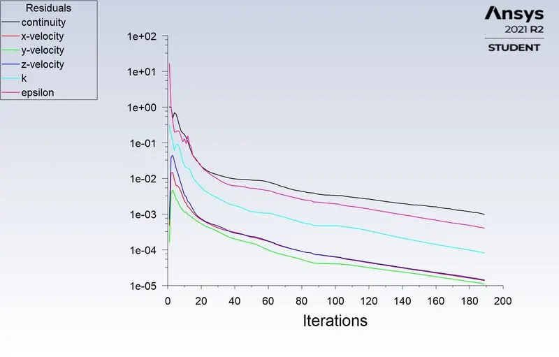
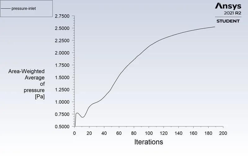
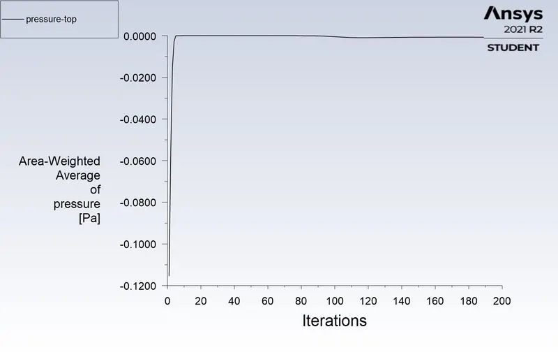
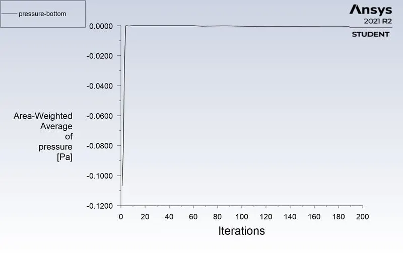
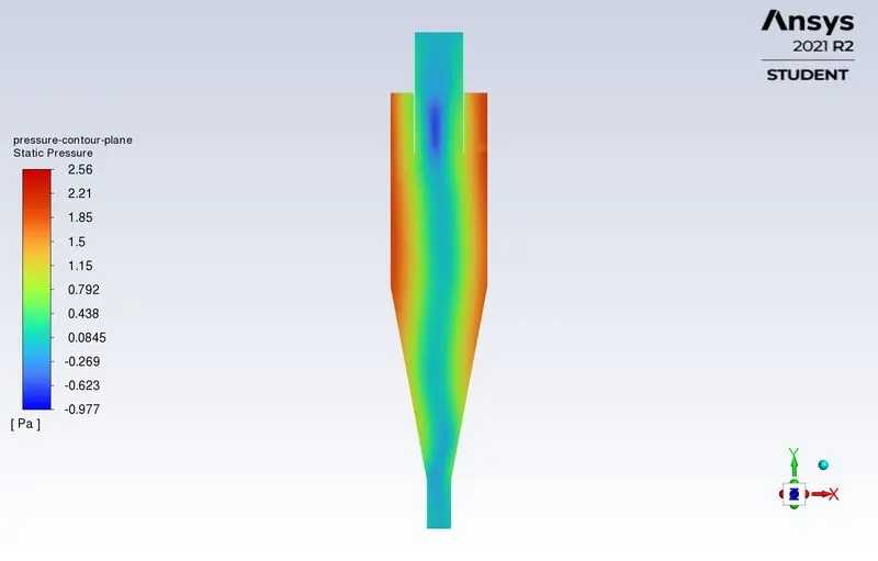
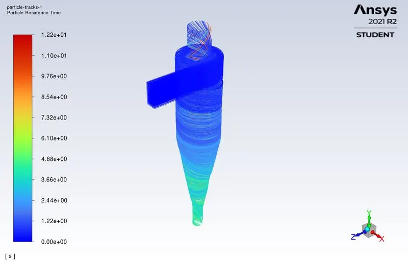
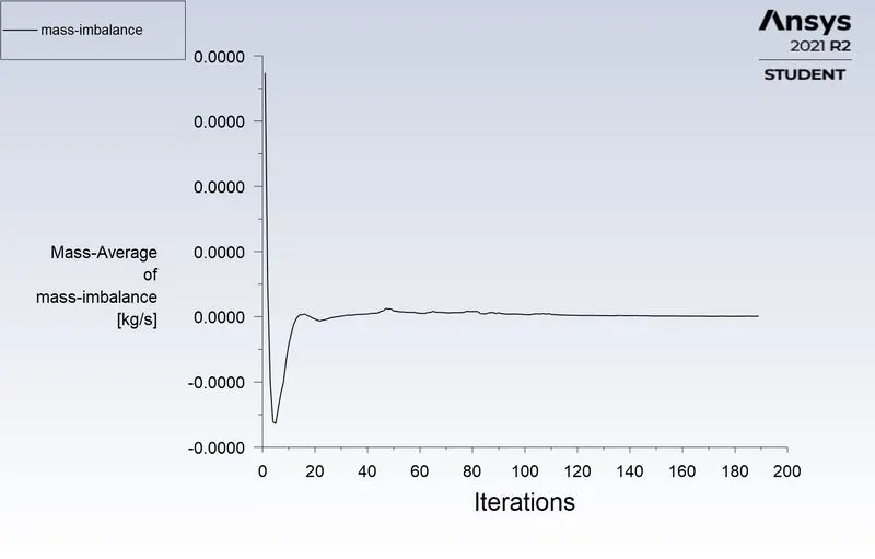
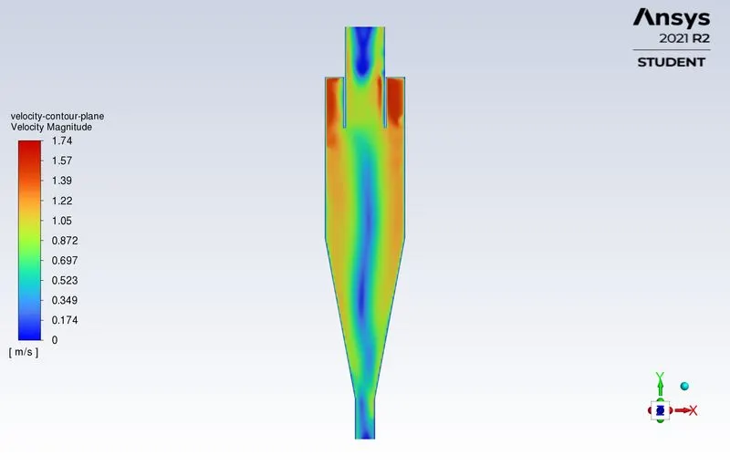
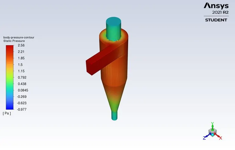
5 Micron 2 meter per second case

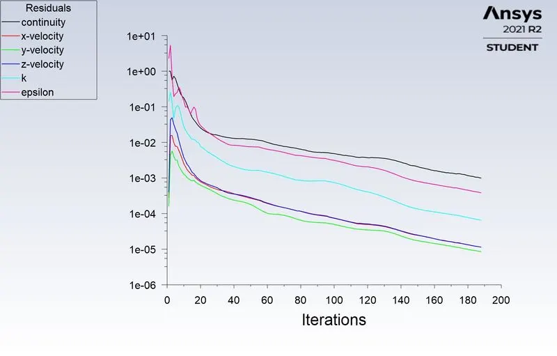
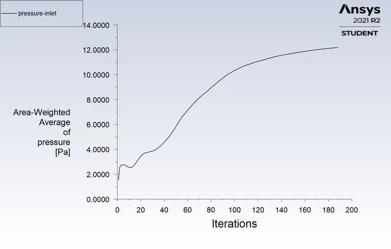
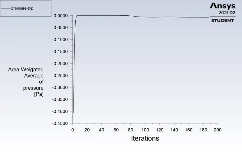
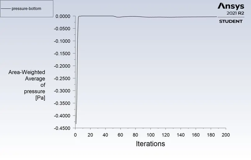
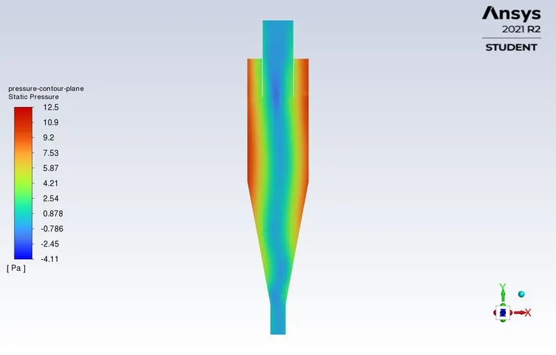
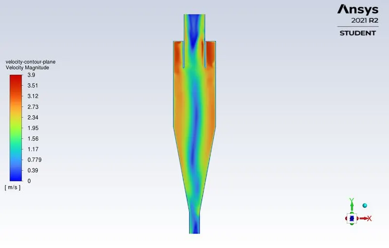
5 micron 3 meter per second case

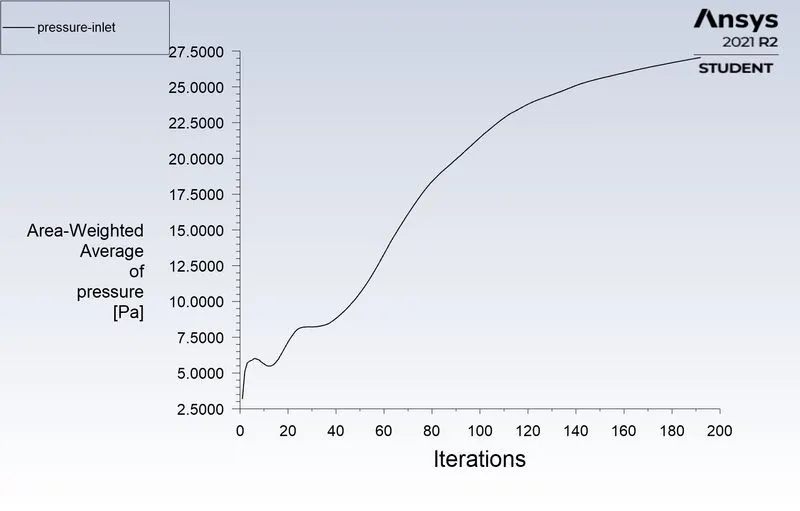
5 micron 4 meter per second case

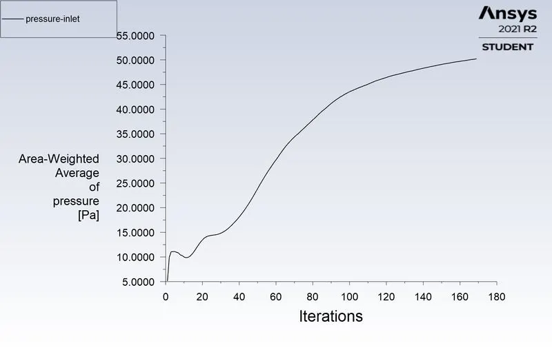
5 micron 5 meter per second case

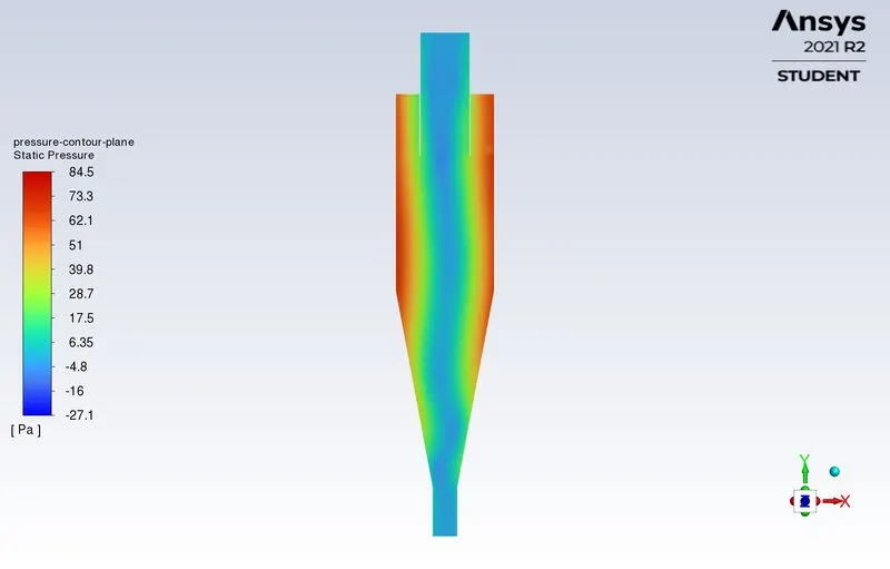
Conclusions:

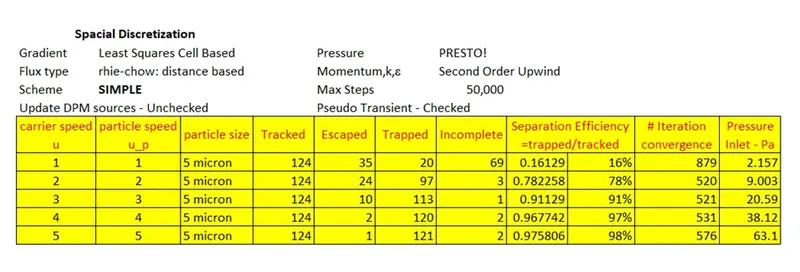
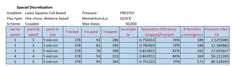
• For the case of a 5-micron particle size, as carrier phase and carrier velocity increases from 1 to 5 meters per second, following conclusions can be inferred –

• Separation efficiency increases with an increase in velocities.
• Pressure difference between inlet and outlets increases as velocities increase, except for the last iteration, with 5 meter per second velocity.

• For the case in which we have a same velocity of 3 meter per second, for carrier phase and particles, we increase particle size from 1 to 5 micron, following conclusions can be inferred –

• The separation efficiency increases with an increase in particle size.
• The pressure difference and rate of convergence remains the same.
• Also, in a generic sense, it can be inferred thus, in SIMPLE scheme, time per iteration is less compared to coupled scheme. On the contrary, in coupled schemes, convergence is achieved with a smaller number of iterations.