Week 8 - Simulation of a backward facing step in OpenFOAM

In this challenge we are asked to simulate a flow of fluid through a Backward facing step, in which the fluid is Incompressible, Laminar and viscous in nature.

The simulation shall be Transient in nature; thus, we shall have to discretize an unsteady Reynolds scalar transport equation for a fluid flow.

Based on the above physics of the flow defined, we will be selecting a specific algorithm to solve for the same.

We have numerous algorithms in Literature to solve various types of flows, namely, SIMPLE, PISO, PIMPLE and a few more. In order to simulate our problem, we shall be selecting the PISO algorithm which has been explained in the ensuing sections.

Selecting the Solver:

We need to choose a solver in OpenFOAM which will be employing the PISO algorithm for incompressible, transient, laminar and Newtonian fluids. Upon perusal of various types of flow simulations in the OpenFOAM tutorials folder, it is found that the icoFoam solver which comes under the incompressible folder is most suitable for this application and flow physics.

icoFoam:

icoFoam is an OpenFOAM solver suitable for analysing incompressible, laminar flow of Newtonian fluids. It is based on the PISO algorithm (pressure-implicit splitting of operators), which is essentially a pressure-velocity iterative procedure for transient problems. In each iterative step, PISO solves the momentum equation using one predictor step, with two further corrector steps for both velocity and pressure.

Objectives

• Basic case setup in OpenFOAM
• Setting up initial values of p and U
• Ensuring proper boundary definitions
• Understanding pressure, velocity files in 0 folder, Transport properties from constant directory and blockMesh Dict, controlDict, fvSchemes and fvSolution from systems directory.

1. Pre-processing

Basic case setup in OpenFOAM:

0 directory

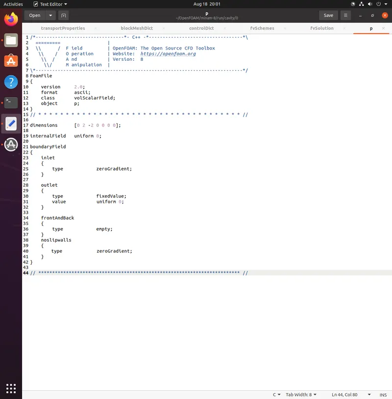
The 0 directory includes the initial conditions for running the simulation. In each file in this folder the initial conditions for one property can be set. The files are named after the property they are standing for, e.g., P file includes pressure initial conditions.

P file can be opened using ‘gedit’ or ‘vim’ or ‘nano’ command in the terminal window in Linux ubuntu in 0 directory.

p stands for pressure and U stands for velocity.

• Understanding pressure file.

In dimensions, the physical dimension according to SI base units of the quantity is defined, for example here it shows that the p dimension is (m/s)².

Note: As you can see the p unit is not the pressure unit (Pa). It is due to the fact that in incompressible solvers in OpenFOAM, p is defined as “reduced” pressure divided by density.

Also, in the dimension matrix the first number represents mass (kilogram), the second one the length (meter), the third one time (second), the fourth one the temperature (Kelvin), the fifth one the quantity (mole), the sixth one current (ampere) and the last one luminous intensity (candela).

`P/ρ=(N⁄m^2 )/(kg⁄m^3 )=Nm/(kg)=((kg-m⁄s^2 )⋅m)/(kg)= (m/s)^2`

The internal Field sets the initial field of a specific quantity in the solution domain. There are two types: uniform and non-uniform. Uniform field assigns a single value to all elements, whereas non-uniform field specifies a unique value to each field element.

The type of each of our boundaries as well as the value of this quantity on the boundaries is defined in the boundaryField. There are different types of boundary conditions in OpenFOAM:

- zeroGradient: Applies a zero gradient boundary type to this boundary (Neumann boundary condition).

- fixedValue: Applies a fixed value to this boundary (Dirichlet boundary condition).

- empty: It is for sides, which are vertical to the direction that is not going to be considered.

• Understanding Velocity file.

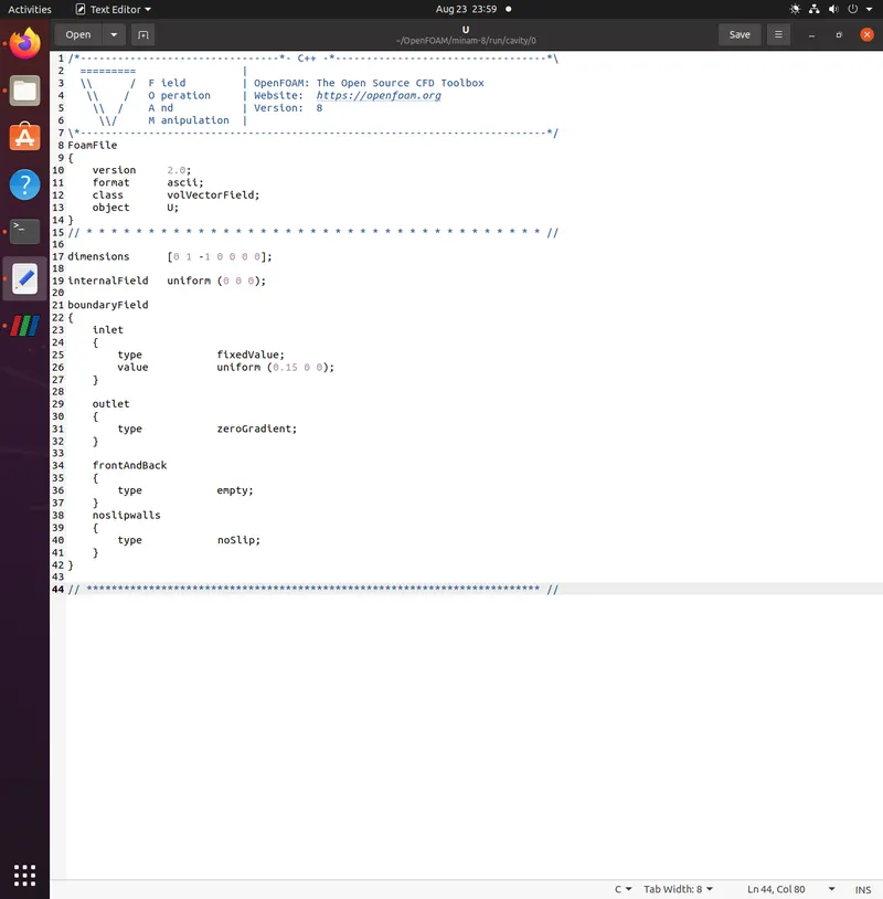
The U file has to be defined via three components (since velocity is a vector): first one stands for the x component, second one for the y component, and the third one for the z component. For this case setup the z component is always zero because it is a 2D simulation and no calculations will be done in the z direction. The boundaries vertical to z direction have been already set to empty.

In the internal field, we have taken value of zero for all directions. The u and v component of velocity will change upon iterations meaning these values, i.e., zero are the initial guessed values.

The dimension of velocity in SI base units is meter per second and can be seen accordingly under “dimensions”.

Under the boundary field section, for the inlet boundary, we need to decide u component of velocity in such a way that our resulting flow is laminar. For that we need to first calculate the Reynolds number.

The Reynolds number in practice

Experiments have shown that in general, Reynolds number values between 2000 and 4000 is the range of transition from laminar to turbulent flow.

Thus, we shall be limiting our Reynolds number to a value of less than 2000.

The Reynolds Number formula is: “Re = ρVD/μ” or “Re = VD/v” where “V” is the fluid velocity, “D” is the characteristic distance, “ρ” is the fluid density, “ν” is the kinematic viscosity, and “μ” is the dynamic viscosity

“D” is also called Hydraulic Diameter and is equal to 4 times the cross-sectional area divided by wetted parameter.

Based on the geometry, the hydraulic diameter for the 2 sections is calculated to be 0.01 meter and 0.0133 meter for the smaller and bigger section respectively.

Taking larger of the two values, the velocity comes to about 0.15 meter per second.

This value, when approached in a logical manner, does make sense as the total length of the domain under analysis is 0.20 meter or 20 cm. A velocity of 0.15 m/s or 15 cm/s for 2 or 3 seconds should keep the flow laminar in nature.

Thus, we will give our u component of velocity a value of 0.15 m/s.

constant directory

The constant directory usually consists of a subdirectory and some files. The files (usually) include material properties, simulation physics and chemistry.

In the directory “polyMesh” the mesh data are stored (in this case the data for converted mesh). The boundary file in this polyMesh directory includes the mesh boundary data, e.g. type, the patch group, number of faces on this boundary and also starting face.

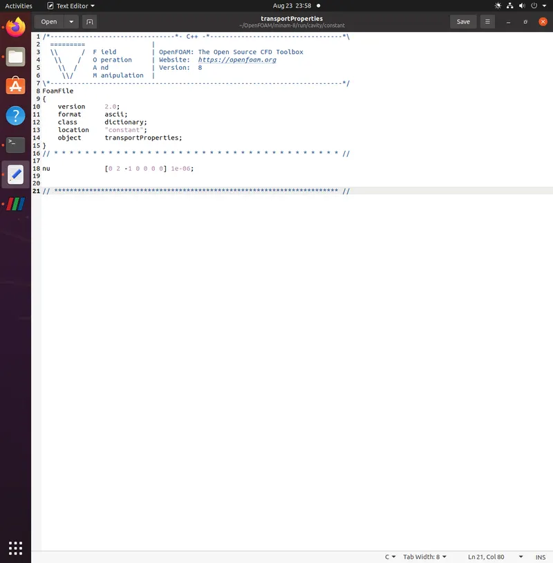
By opening the transportProperties file, properties dimensions and also the property value can be found and edited.

The dimension of kinematic viscosity in SI base units is square meter per second and can be seen accordingly in the line below.

e.g.: nu [ 0 2 -1 0 0 0 0] 1e-6;

nu is the fluid kinematic viscosity, which is 1e-6 m²/s for this example since we have considered the fluid to be water.

A google search for the kinematic viscosity of water gives us a value of 1 mm²/s which equals to 1e-6 m²/s.

system directory

Solver and finite volume methods settings can be found and changed in this directory. There are three main files in this directory:

fvSchemes: The discretization scheme which is used for each term of the equations are set in this file

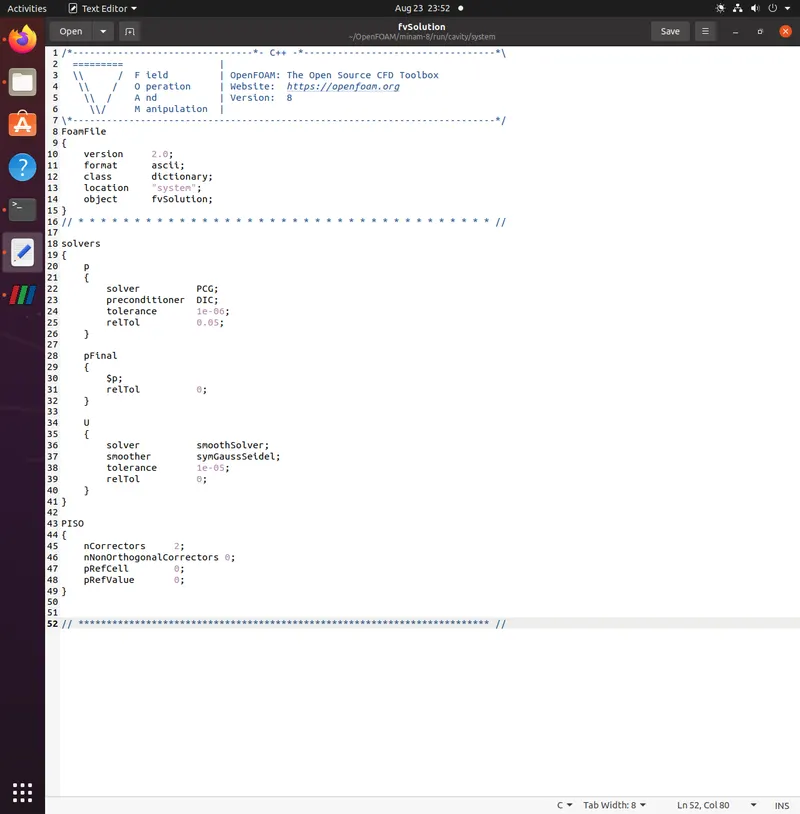
fvSolution: Contains the settings to the coupling method of pressure and velocity, the numerical methods, which are used for solving different quantities, and also the final tolerance for convergence of that quantity.

controlDict: The time from where simulation starts (startFrom), the time when the simulation finishes (startAt), the time step (deltaT), the data saving interval (writeInterval), the saved data file format (writeFormat), the saved file data precision (writePrecision), and also if changing the files during the run can affect the run or not (runTimeModifiable) are set in this file.

blockMeshDict : Here we define the vertices of the geometry.

Note:

If the write format is ascii, then the simulation data which is written to the file can be opened and read using any text editor. If the format is binary, the data will be written in binary style and is not readable by text editors. The advantage of binary over ascii is the smaller file size, and consequently faster conversion and writing to disk, for big simulations.

• Understanding “blockMeshDict”

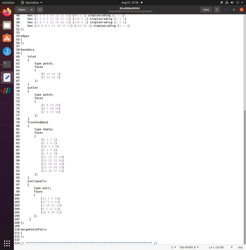
blockMeshDict with a grading factor of 1

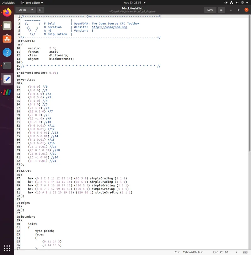
“blockMeshDict” script is used when the meshing needs to be done inside OpenFOAM. For this purpose, the blockMesh tool is used. blockMesh reads the geometry and mesh properties from the blockMeshDict file.

Units used in OpenFOAM are SI units. If the vertex coordinates differ from SI, they can be converted with the convertToMeters command. The number in the front of convertToMeters shows the constant, which should be multiplied with the dimensions to change them to meter which is the SI unit of length. For example:

convertToMeters 0.01

shows that the dimensions are in centi-meters, and by multiplying them by 0.01 they are converted into meters.

In the vertices part, the coordinated of the geometry vertices are defined, the vertices are stored and numbered from zero, e.g., vertex (0 0 0) is numbered 0 and vertex (20 0.5 0) is numbered 7.

In the block part, blocks are defined. The array of numbers in front of each block shows the block building vertices, e.g., the first block is made of vertices (0 1 2 3 11 12 13 14).

After each block the mesh is defined in every direction. E.g., (80 5 1) shows that this block is divided into:

• 80 parts in x-direction.
• 5 parts in y-direction
• 1 part in z-direction.

The reason behind taking a part in z-direction is that even for 2D simulations the mesh geometry should be 3D, but with one cell in the direction, which is not going to be solved. Here 2D simulation is in x-y plane.

The last part, simpleGrading (1 1 1) shows the size function.

In the boundary part each boundary is defined by the vertices it is made of, and also its type and name are defined.

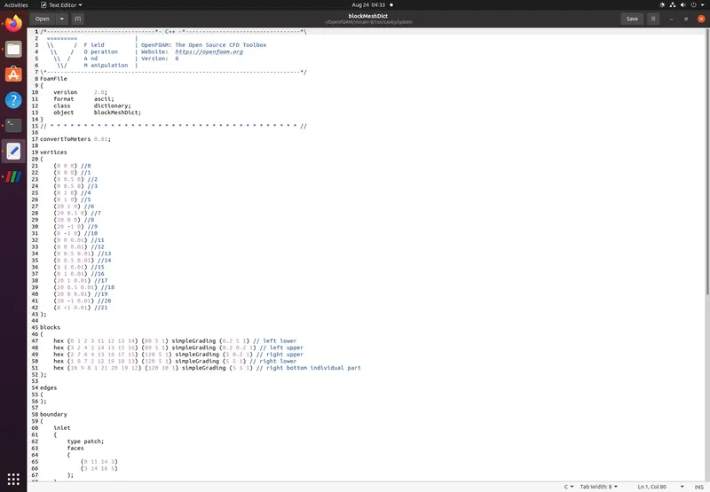
blockMeshDict with a grading factor of 0.2

grading factor is defined as the ratio of cell size at the outflow to the inflow in terms of x-direction.

For the case of Y-direction, it is the ratio of cell size at top to size at the bottom.

In case 2, we have taken a grading factor of 0.2 instead of 1 to observe any changes in flow simulations, velocity profile or any other (these are mentioned in the ensuing paras)

All the cells in between the extreme end cells are divided uniformly throughout.

As can be seen from the blockMeshDict file for Grade factor of 0.2, grading is done to create finer mesh at the walls as the flow near the walls are irrotational as viscosity plays an important role in this region.

Note:

From X = 0.08 till the end, finer mesh at Y = 0 location is not required but we need to take the same as these lines must coincide with the Y lines from the first part of the geometry (X =0 till 0.8 m). This is because any mismatch in lines will lead to improper numerical flow of flux across the faces leading to computational errors and solution returns an error.

For creating a face, the vertices should be chosen clockwise when looking at the face from inside of the geometry.

• Understanding “controlDict”

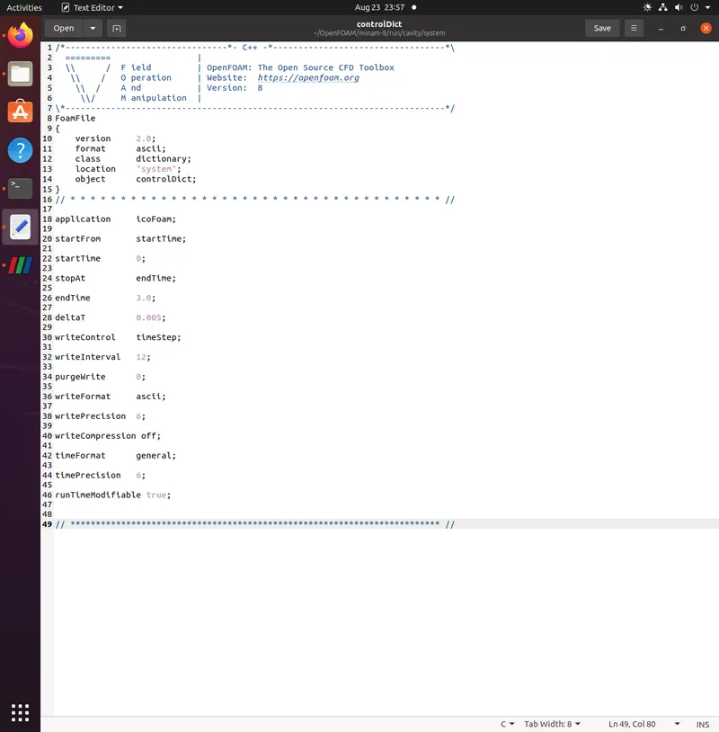
controlDict with a grading factor of 1

Reason for choosing a specific time step (delta T) and end time:

We have created meshes with 200 cells in x-direction. However, one cannot simply increase the number of cells (i.e., decrease the cell size) without changing the time step size accordingly. This is because when running a numerical scheme (e.g., the Gauss linear scheme) the solution is reached using the information propagated by waves or particles from one cell to the adjacent cell. To ensure a physical solution it is essential that the physical flow information e.g., velocity, composition, etc is received by all cells with in the calculation domain. It needs to be guaranteed that the information transport does not “overtake” the physical transport, otherwise the scheme will be unable to access the information required to form the solution. The above criterion is known as the Courant-Friedrichs-Lewy (CFL) condition, and it is a necessary condition for convergence. For one-dimensional problems, it can be written as:

Even though our problem is 2D in nature, I am considering a 1D formula as our flow is laminar in nature.

The key dimensionless number here is the Courant number, , which needs to be less or equal to one.

As it is obvious from the equation by decreasing the mesh size (i.e., ), the time step size ( ) should also be adjusted (decreased) for reaching a stable and convergent solution. Therefore, the CFL condition is useful in helping us choose a suitable time step size for our simulation.

Since we have taken 200 cells in x-direction, our mesh size in x-direction shall be 0.001 meter.

For a velocity of 1 meter/sec, we get a time step size of 0.001 seconds.

But as discussed earlier, in order to maintain a laminar flow, we have chosen a velocity of 0.15 m/s.

For a courant number of 1, mesh size of 0.001 and velocity of 0.15, we get time step size of 0.00667. we can change this value to a lesser value to reduce courant number less than 1 in order to ensure convergence and boundedness. Thus, choosing a value of 0.005 as time step size.

In summary, for a velocity of 0.15 m/s, mesh size of 0.001 meter and time step of 0.005 sec, we get the courant number as 0.75 which is less than 1.

The end time selected is 3 seconds as domain length is 20 cm, and velocity is 15 cm/s, so in 3 seconds we cover a distance of 45 cm ensuring proper flow visualization through domain in the post processing stage.

Write interval has been changed to 12 from 20.

Based on delta T value and time step size, we know that the number of time steps shall be 600. Displaying of all 600-time steps is redundant and not required. In order to keep things simple, we shall keep only fifty (600/12=50) time folders excluding 0, constant and systems directory. Thus, write interval has been changed to 12.

Time precision is 6, which accepts 6 digits after the decimal. This is related to accuracy.

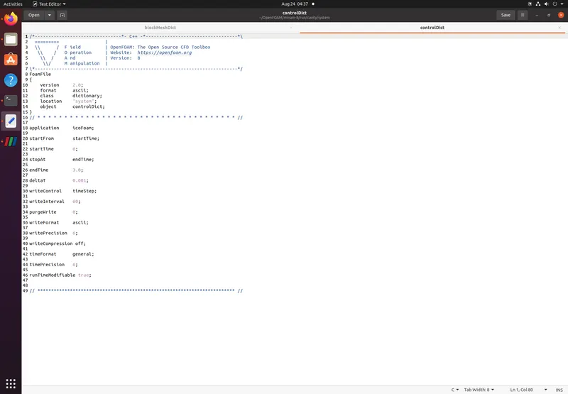
controlDict with a grading factor of 0.2

Of course, as the mesh size changes, so should the time step size change accordingly.

Here, the smallest mesh in x-direction is 20 percent of the mesh size as calculated from grading factor of 1. Thus, our smallest size of mesh shall be 0.0002 meter.

Keeping the courant number as 1, with a u component of velocity of 0.15 m/s, mesh size of 0.0002, we get the time step size of 0.00133 s.

Taking a time step size of 0.001 seconds, we get courant number of 0.75. The solution now does not blow up!

Write interval has been changed to 60 from 20.

Based on delta T value and time step size, we know that the number of time steps shall be 3000. Displaying of all 3000-time steps is redundant and not required. In order to keep things simple, we shall keep only fifty (3000/60=50) time folders excluding 0, constant and systems directory. Thus, write interval has been changed to 60.

The execution time in the terminal for this case is more than the previous case as now we have 3000-time steps instead of 600.

A screenshot of the controlDict file for both the grade factors have been shown in images.

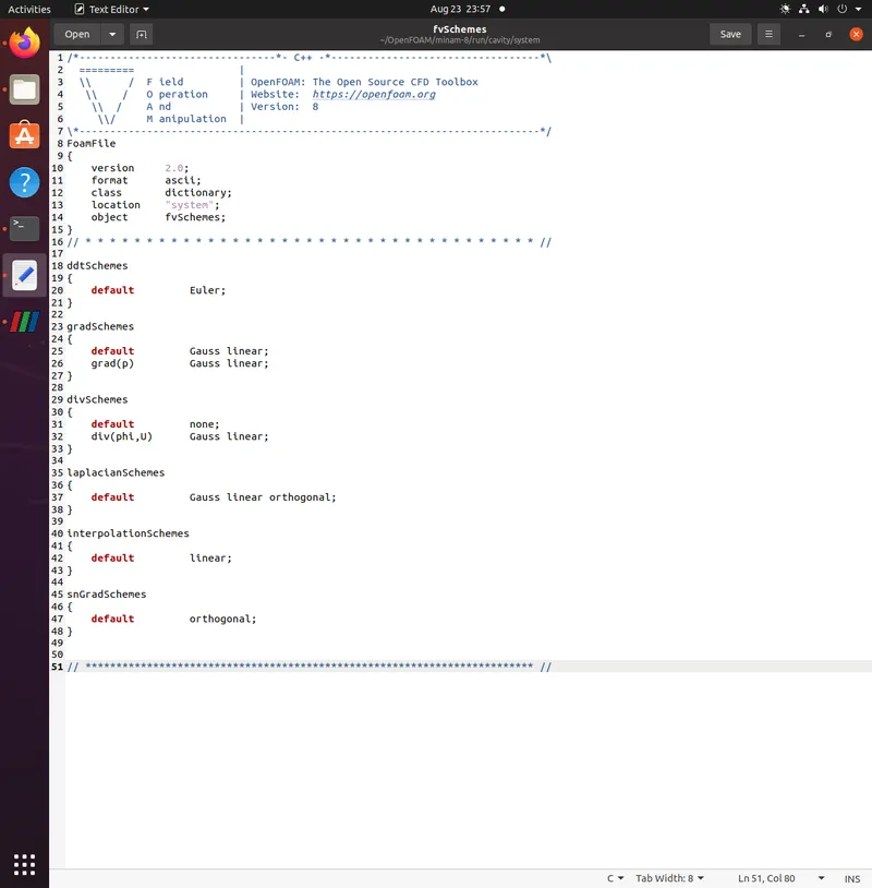
• Understanding “fvSchemes”

For each type of operation, a default scheme can be set (e.g., divSchemes is set to none, it means no default scheme is set).

Also a special type of discretization for each element can be assigned (e.g. div(phi,U) it is set to Gauss linear). For each element, where a discretization method has not been set, the default method will be applied. If the default setting is none, no scheme is set for that element and the simulation will crash.

Note:

In fvSchemes, the schemes for the time term of the general transport equation are set in ddtSchemes sub-dictionary. divSchemes are responsible for the advection term schemes and laplacianSchemes set the diffusion term schemes.

divSchemes should be applied like this: Gauss + scheme. The Gauss keyword specifies the standard finite volume discretization of Gaussian integration which requires the interpolation of values from cell centres to face centres. Therefore, the Gauss entry must be followed by the choice of interpolation scheme

• ddtSchemes – Euler (default)

Discretization of the time derivative of the transport equation is performed by integrating it over the control volume of a grid cell.

Here, the Euler implicit time differencing scheme is used. It is unconditionally stable, but only first order accurate in time. Assuming linear variation of φ within a time step gives:

• grad Schemes – Gauss linear

in our fluid flow equation discretization, we have the term grad p as shown below, this term needs to be interpolated after applying the gradient theorem (green gauss theorem)

linear stands for linear interpolation of values from cell to face centres and in literature, is also called as the central differencing method, which has been discussed in detail in week 9 challenge of the same module.

• Divergence Schemes – Gauss linear

Similar to grad scheme, we shall be using the gauss linear method to discretize the divergence term which is the convection term in the fluid flow transport equation.

Div(phi,U) in this, phi is rho times velocity vector. In terms of partial differential form, it is

• Laplacian scheme and sn grad Scheme – Gauss linear orthogonal and orthogonal

It is worth explaining the snGradSchemes sub-dictionary that contains surface normal gradient terms, before discussion of laplacianSchemes, because they are required to evaluate a Laplacian term using Gaussian integration. A surface normal gradient is evaluated at a cell face; it is the component, normal to the face, of the gradient of values at the centres of the 2 cells that the face connects.

As our mesh is cartesian mesh, our surface normal shall be orthogonal in nature.

The laplacianSchemes sub-dictionary contains Laplacian terms. A Laplacian term is the diffusion term in the momentum equations, which corresponds to the keyword laplacian(nu,U) in laplacianSchemes.

The Gauss scheme is the only choice of discretisation and requires a selection of both an interpolation scheme for the diffusion coefficient, and a surface normal gradient scheme.

To summarise, the entries required are:

Gauss <interpolationScheme> <snGradScheme>

• Interpolation Schemes

The interpolationSchemes sub-dictionary contains terms that are interpolations of values typically from cell centres to face centres, primarily used in the interpolation of velocity to face centres for the calculation of flux phi.

• Understanding “fvSolution”

Understanding solvers in this case would require an in-depth study which was not undertaken during the course of this challenge, but very briefly, solver used for pressure is called the PCG solver which is an iterative conjugate gradient solver. It is the most robust solver and is recommended for nonlinear problems.

• Running Simulation

The simulation can be run by typing the solver’s name in the cavity folder and executing it:

>icoFoam

Note:

For running the simulation, the solver command (e.g., icoFoam) should be executed inside the copy of the tutorial main folder. The command should be executed in the cavity folder, if it was run at some subfolders or somewhere else, the simulation will fail.

Notable observations:

1. After making all the necessary modifications in blockMeshDict file, “blockMesh” command needs to be executed in terminal to update the mesh defined as per blockMeshDict file.
2. Number of correctors in fvSolution file is set to 2 as PISO algorithm has 1 predictor and 2 corrector steps.

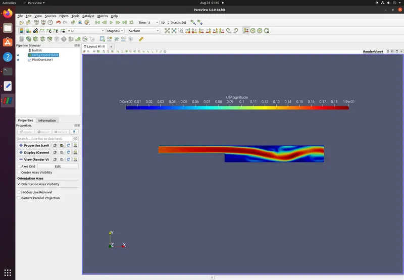
• Fluid flow shot for a Grade Factor of 1

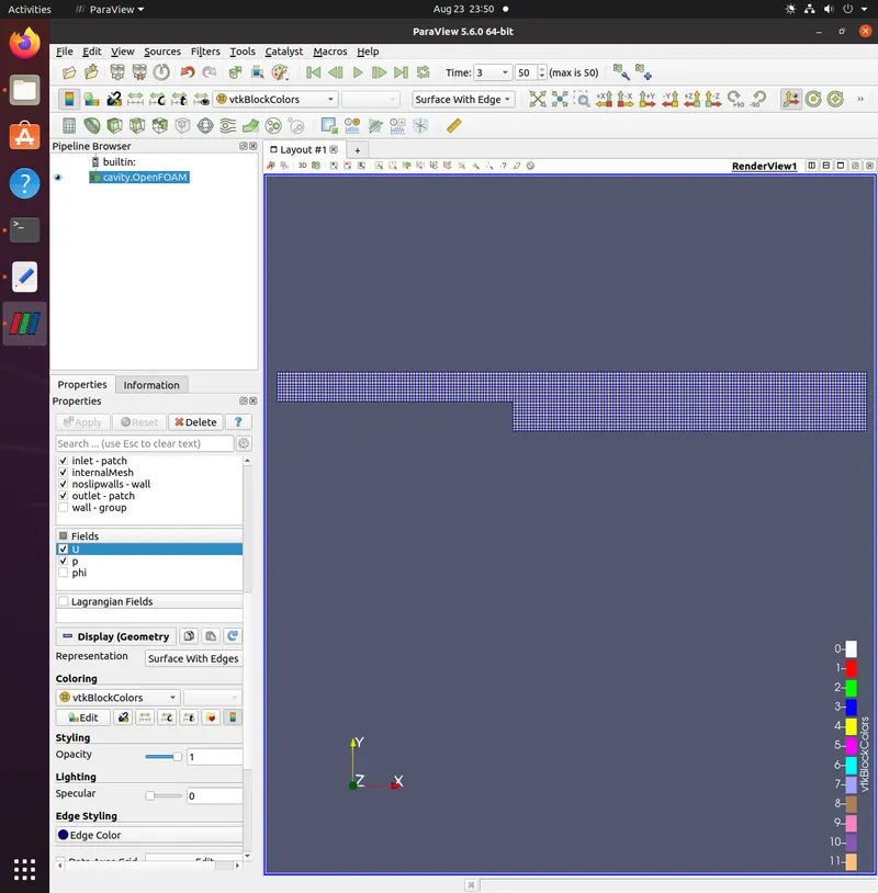
• Mesh outline using Grade Factor of 1

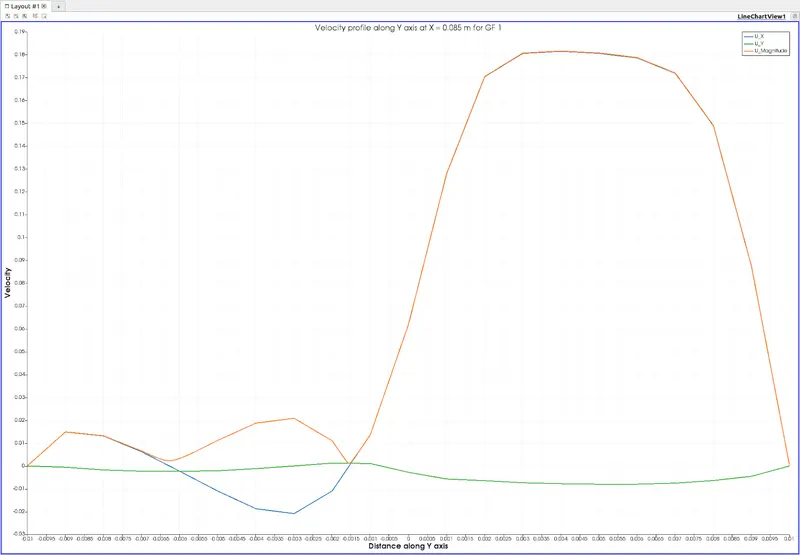
• Velocity profile along Y axis at X = 0.085 m for grade factor 1

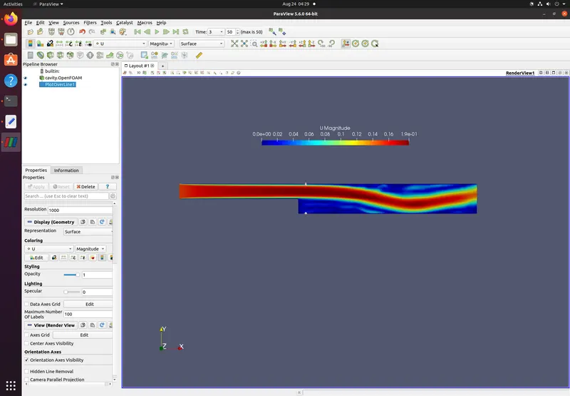
• flow simulation for GF 0.2

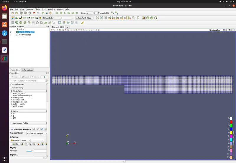
• Simple grading with Grade Factor of 0.2

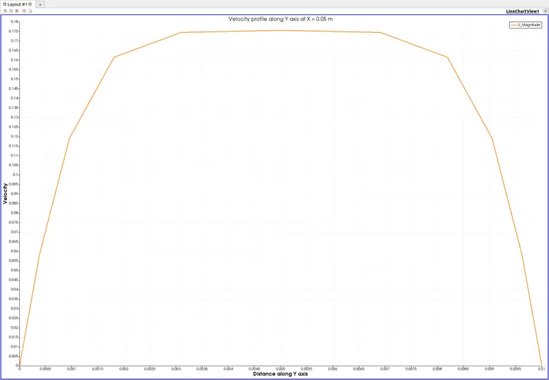
• velocity profile at X = 0.05 m

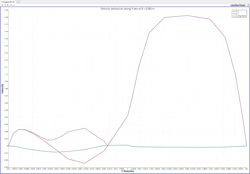
• Velocity profile GF 0.2 at X = 0.085 m

Comments and Conclusions:

1. As we changed the grading factor from 1 to 0.2, the size of the mesh reduced. This required a change in the time step size as the courant number value increased to a large magnitude resulting in termination of the solver.
2. Change in time step size and the value chosen is explained above in the report.
3. Plots have been attached which show a variation of velocity along Y axis at location of X = 0.05 meter, this is the location were the flow is completely laminar without experiencing flow separation, irrotational flow etc which is experienced later at the step.
4. These plots for both GF of 0.2 and 1, show us that the velocity profile is parabolic in nature. This is in lieu of what was taught in fluid mechanics literature for a plane Poiseuille flow.
5. A closer look at the plot shows us that the maximum velocity occurs at the centre line, i.e., 0.05 from bottom and top.
6. The maximum velocity at the centre line is greater than the value taken by the user. User specified value of velocity is 0.15 meter (this specific value was taken to ensure a laminar flow, the explanation of the same is noted in the report).

A total of 50 folders are written by taking writeinterval as 12 and 60 for Grade Factor of 1 and 0.2 respectively.

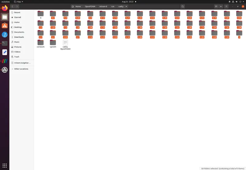
This is a collage of 2 seperate videos using Grade Factor of 1 and 0.2.