Week 5 - Rayleigh Taylor Instability
OBJECTIVE:
The objective of this challenge is to simulate a two-dimensional Rayleigh-Taylor instability problem.
INTRODUCTION:
In Multiphase flows, the dynamic variables like velocity, pressure, viscosity, density etc are the driving members for movement of fluids under gravitational field. One such example is of Rayleigh-Taylor Instability.
It is a hydro-dynamic Instability which arises when a high-density fluid is placed oven a low-density fluid in a gravitational field.
The RTI (Rayleigh-Taylor) phenomenon was initially introduced by Rayleigh in 1883 and later was observed for all accelerated fluids by Taylor in 1950. When the density interface is disturbed, hydrostatic pressure is generated, so the heavier fluid moves downwards and mixes with the lighter fluid, with the amplitude of perturbation growing exponentially but after sometime saturates and forms characteristic mushroom shape.
When a heavier fluid is displaced downwards with an equal volume of lighter fluid being displaced upwards, it results in decrease of potential energy than its initial state.
As the RT instability develops, the initial perturbations progress from a linear growth phase into a non-linear growth phase, eventually developing "plumes" flowing upwards (in the gravitational buoyancy sense) and "spikes" falling downwards. In the linear phase, the fluid movement can be closely approximated by linear equations, and the amplitude of perturbations is growing exponentially with time. In the non-linear phase, perturbation amplitude is too large for a linear approximation, and non-linear equations are required to describe fluid motions.
In general, the density disparity between the fluids determines the structure of the subsequent non-linear RT instability flows (assuming other variables such as surface tension and viscosity are negligible here).
The difference in the fluid densities divided by their sum is defined as the Atwood number, A.
For A close to 0, RT instability flows take the form of symmetric "fingers" of fluid; for A close to 1, the much lighter fluid "below" the heavier fluid takes the form of larger bubble-like plumes.
We shall have a look at the same in our post-processing results.
Real life applications:
Applications of RTI can be witnessed in wide range of problems including the mushroom clouds like volcanic eruption and nuclear explosion.
In this study the 2D geometry is itself constructed in Space claim and a computational mesh is generated. The meshing file is imported in fluent and a grid dependency test was performed for a mesh size of 0.1 mm and 0.05 mm and the results of the interfacial evolution of RTI is captured at different flow times.
The spatial discretization involves least square cell based for gradient and for time derivative, first order implicit scheme was used in order to solve the governing equations, as implicit scheme is unconditionally stable.
SIMPLE scheme was employed to overcome the pressure velocity coupling. In this study the density of the secondary phase is altered with the incorporation of user defined material resulting in variation of Atwood Number. Density and viscosity chosen is 400 kg/meter square and 0.001 kg per meter-second.
The results of the grid dependency study and the variation of Atwood Numbers are carefully observed and reported.
Pre-processing and Mesh
At first, geometry is created as square boxes and converted to surface using Pull tool and share topology is turned on. The geometry was created in spaceclaim and it involves no other importing of CAD models. The surface model was further processed for meshing and the results were taken for three different meshing schemes. This pre-processing phase of the workflow is extremely important because it determines the simulation potential and limits the CFD results.
Case A – Water-Air
Mesh details:
Baseline mesh – 0.5 mm
Element size: Elements – 2000
Case B – Water-Air
Mesh details:
Mesh – 0.1 mm
Element size: Elements –80,008, Nodes – 80,606
Case C – Water-user defined fluid
Mesh details:
Mesh - 0.25 mm
Element size: Elements – 12500
CFD Case Setup
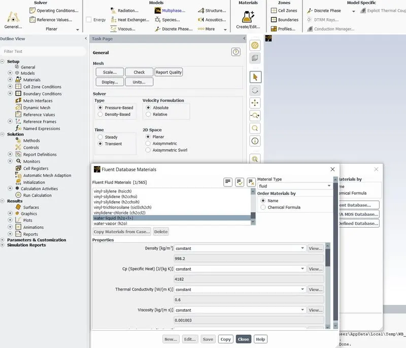
- Pressure based solver and Absolute velocity is used.
- Transient-state calculation is performed.
- Compressible fluid flow is chosen.
- Gravity is enabled in negative Y axis – 9.81 m/s2.
- Multiphase Model is turned on along with Volume of Fluid and number of Eulerian phases is chosen as 2 and Implicit scheme is selected.
- Viscous Model used – Laminar.
- Patching of the volume fraction of the two phases is performed before the start of simulation. Phase used for patching was water and volume fraction of 1 is taken for water surface and 0 for air surface.
- In Pressure velocity coupling SIMPLE scheme is used. For the momentum second order upwind scheme is used and for pressure, PRESTO is selected. For the transient formulation first order implicit scheme is chosen for better results and for stability and convergence of the residuals.
Stages of development and evolution into turbulent mixing, method of choosing time steps and calculation procedure – Air-water setup:
Phase 1 of video
In first phase of simulation, under time advancement, an adaptive type of advancement was chosen with global courant number equal to 1.5.
By default, in FLUENT, the global courant number is 2, but smaller value may be required for more accurate solution and more stable numerical calculation. In some cases, you need to reduce this up to 0.5 for accurate results and this is because the time step size (so, the CFL) should be small enough to get the accurate results.
Also, the initial time step size chosen was 0.001, which reduces even further if the global courant number for any time step increases above any stipulated value set by fluent (need to understand some more on this). In our simulation, after a few time steps, the global courant number increased to about 15. Thus, the time step size kept on reducing till it reached a value in the range of e-5. This saves the simulation from blowing up, but also increases the computational time and cost considerably.
Other method is to assume an educated fixed time step size and see if the solution does not diverge. If it does, then repeat the calculations with reduced time step sizes. However, this method is taken care of by choosing an adaptive style of time advancement which was done in this challenge for about 100-time steps (a side effect of which is of course, very low values of step sizes if courant number increases).
Now, an important point to remember is the flow time, which is the product of time steps and step size. A direct corollary of step size reduction is reduction in flow time simulated/analysed. This of course, increases the number of time steps to reach an equilibrium eventually increasing the simulation time and computation cost.
Thus, in a nutshell, for first 100-time steps, the following values were taken.
Type of time advancement = Adaptive
Initial time step size = 0.001
Global courant number = 1.5
Number of time steps = 100
Phase 2 of video
In phase 2 of video, one can witness an increase in speed of simulation, this was because the global courant number was increased to 0.9, this led to a gradual increase in the step size as the simulation progressed. This was run for about another 200-time steps.
Total time steps at end of phase 2 is 300.
Phase 3 of video
The third phase of video was analysed for about 1600-time steps with fixed type of time advancement. Time step size chosen was 5e-4 to ensure solution doesn’t blow up. This can be witnessed by an increase in simulation speed.
Total time steps at end of phase 3 is 1900.
Phase 4 of video
Next phase of video was run for about 630-time steps with yet an increased time step size of 0.001. The reason for gradually increasing step size every few time steps is to ensure solution does not blow up, as is evident from literature that solution blows up for finer meshes, at beginning of simulation. This can also be understood by the fact that step sizes reduced in the first 300-time steps with adaptive type of time advancement.
Phase 4 ends at 2530-time steps.
Phase 5 of video
This phase was run for almost the remaining entirety of simulation at time step size of 5e-3.
A few of ending time steps were run at 0.1 delta t values to increase flow time and ensure an equilibrium condition. This though, cannot be visualised from the video as the changes are negligible.
Atwood number in this case = 1000-1.2 / 1000+1.2 ~ 0.9
Plots on water volume fraction:
Initially, the perturbation amplitude is smaller compared to wavelength.
Equation of motion can be linearized.
Exponential instability growth is witnessed.
Later on, non linear effects begin to appear. This can be seen from mushroom shaped spikes and bubbles.
Spikes: These are fluid structures of heavy density fluid growth into lighter fluid.
Bubbles: These are fluid structures of lighter density fluid growth into heavier fluid.
Disturbance in flow from smooth to turbulent growth has been observed.
In the next shot, we can see a transition of a single globule into lots of deformed globules with lots of turbulence along with some breakup and penetration of heavier fluid into the lighter one.
At later time we observe the formation of low-density bubbles and its rise into the high-density phase whereas the high-density globules sink at the edges of the domain of the simulation into the light fluid.
Snippets from workflow have been attached for reference...
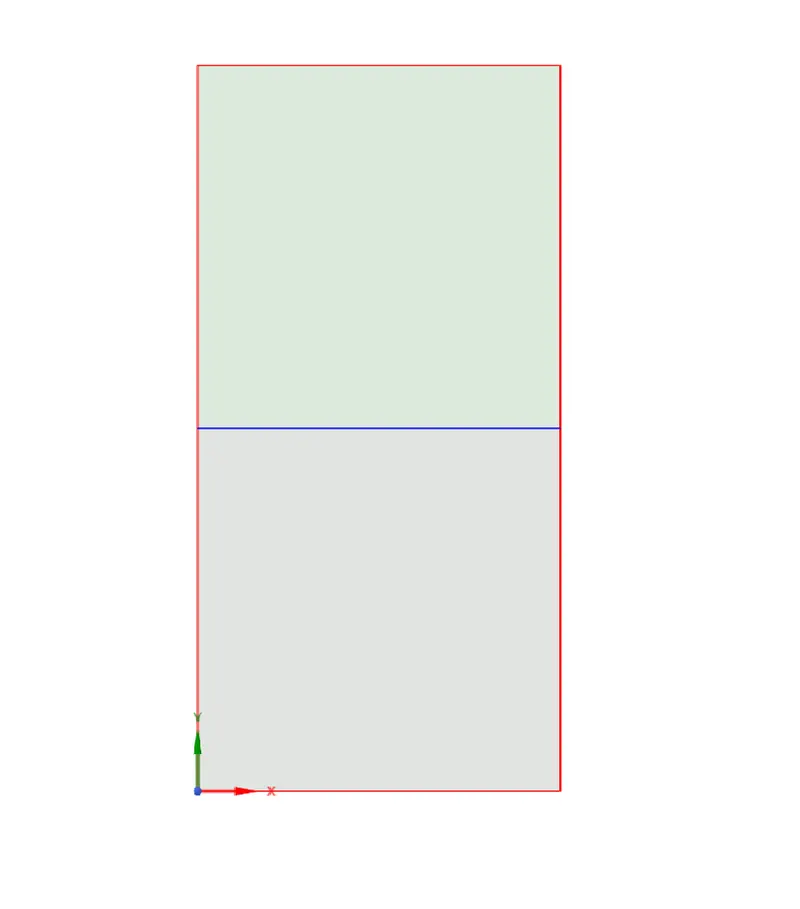
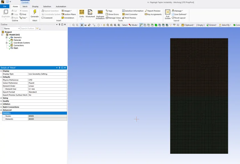
Meshing - Refined Case Setup
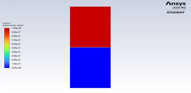
Volume of Fluids
Stages of development and evolution into turbulent mixing, method of choosing time steps and calculation procedure – Customised fluid-water setup:
For the case of a user defined and water setup, a customised fluid (user defined) with density of 400 kg per squared meter was modelled in fluent. This user defined fluid is kept at the bottom portion with water in the top portion of geometry.
The Atwood number in this case is calculated as shown below:
A = 1000-400 / (1000+400)
A = 0.42
As Atwood number is closer to 0, thus in this case we see finger like forms in the initial stages of simulation as opposed to plumes rising up in case where Atwood number is closer to 1 due to more pronounced density difference.
Here the simulation was run choosing a fixed type of time advancement with a time step size of 0.005.
Mesh size was increased to 0.25 mm to reduce the computation time, although at an expense of simulation run clarity. The simulation plots look more diffused and smudged as compared to the refined case of air and water setup.
Adaptive type of time advancement was not used to save computational time.
This simulation was run for abount 1500*0.005 = 7.5 seconds in real time. Although the computation took about 20-25 minutes which was still was lower than using the adaptive technique!
Playing around with time steps in Part 1 of this challenge took about 6 hours. This of course also depends upon the hardware being used but is seriously hampered when using a student version which limits the user to simulate any simulation using upto 4 processors in parallel.
Why a Steady state simulation might not be appropriate?
Transient solver better captures the flow and can be used to run at smaller time steps which is seen from part 1 of this challenge adopting various sizes of time steps as discussed above to avoid blowing up of solution.
Smaller time steps are required to observe the instabilities and can only be possible through transient simulations.
Since it is a time marching solution, we expect more accuracy from transient simulation to run calculations for Rayleigh Taylor Instability.
Conclusion:
- For the case of smaller Atwood Number, the density difference between the two sides of the interface is small and the density distribution of the upper and lower layers is nearly symmetrical.
- The initial density stratification plays a dominant role and the expansion compression effect has a little influence.
- With the increased Atwood Number close to 1 the stabilization effect of initial density stratification decreases and the instability caused by the expansion-compression effect becomes more significant.
- At Atwood number close to 1, larger amplitude of perturbation can be witnessed.
- It takes place due to the larger density ratio of two fluids, stronger forces develop the interface instability.
- In case of Atwood number closer to 1, the time of spikes or globules of the lighter phase fluid arriving at the bottom of the computational domain is accelerated.