Week 1- Mixing Tee

Aim

• To set up steady state simulations in order to compare mixing of hot and cold fluid through outlet of a geometric tee model.
• Given 2 cases, were in two versions of a mixing tee have been modelled. Need to use k-epsilon and k-omega SST model for case 1 and based on the judgement, use only one method accordingly in case 2.
• The 2 cases are stated below.

1. Case 1(a) –

• Short mixing tee with hot inlet air velocity of 3 meter per second and cold velocity of 6 m/s.

2. Case 1(b) –

• Short mixing tee with hot inlet air velocity of 3 meter per second and cold velocity of 12 m/s.

3. Case 2(a) –

• Long mixing tee with hot inlet air velocity of 3 meter per second and cold velocity of 6 m/s.

4. Case 2(b) –

• Long mixing tee with hot inlet air velocity of 3 meter per second and cold velocity of 12 m/s.

Expected Results:

Plot velocity and temperature contour and line plots along and across the length of pipe.

Perform Mesh Independent study and discuss the effect of length and momentum ratio as a conclusion.

Introduction:

Before we start with analysing various cases, let us try and understand the two proposed methods, k-epsilon and k-omega SST.

K-epsilon and K-omega SST Model:

In order to have a better understanding on the k-omega SST model, we need to know the fact that k-epsilon and k-omega models were developed earlier, and the k-omega SST model was developed later on as an improvement on these original models.

k-epsilon model was developed first and it was found that the damping functions from this model becomes unreliable for some specific flows and differ in behaviour from real life applications.

In response to this, the k-omega model was developed to give better near wall behaviour that is less sensitive and does not require near wall damping functions.

But now it was found that the solution values for the k-omega model were actually sensitive to the free stream values of the turbulence applied at the inlet to these computations.

But these were typically for the external aerodynamic flows, such as flow over an aerofoil etc, were lift and drag were affected.

Thus, for k-epsilon and k-omega model, it was found that the flow was not separating correctly from surface of the body as compared to experimental data.

Reason for this was attributed to very high values of wall shear stress.

This led to the inception of the k-omega SST model by ‘MENTOR’ in 1994 in order to try and rectify these issues.

A brief view of k-epsilon model without falling into the details of equations.

We have transport equations for turbulent kinetic energy ‘k’ and also for the turbulent dissipation rate ‘epsilon’.

From papers, I have found out that the value of epsilon is written as C_mkw and then substituted into the transport equation for turbulence dissipation rate.

This gives us an additional term, which is not found in the k-omega model.

When this additional term is multiplied by (1-F1), we get to transition smoothly between the k-epsilon and k-omega model by appropriate selection of F1.

For F1 = 0, model is k-epsilon

For F1=1, model is k-omega.

This F1 is called the blending function.

This means that F1, based on our understanding from before, takes on a value of 1 near wall and 0 away from the wall. And takes on the values between 0 & 1 for cells in the transition zone, i.e., not very near or far off from the walls in order to attain a smooth transition between the two models.

The k-omega SST model in itself, has undergone some changes in terms of the blending constants taken from emperical relations, these changes have been incorporated in the softwares we use, the latest version being the wilcox version established in the year 2006.

So which model should we use in this challenge??

The k-omega SST model gives better agreement with experiments of mildly separated flows as found out by mentor and a succession of other authors.

This is particularly important for external aerodynamic applications such as wing or aerofoil, so results of the solution are quite sensitive around the separation point which will determine when stalling takes place eventually affecting the performance of the product.

Our product in focus (mixing tee) in a sense, has no region of flow separation along walls of the tee. And we are not trying to predict the separation point in this case.

We need to analyse and determine the mixing effectiveness of the mixture at the outlet of the tee.

As a final conclusion, k-omega SST model is the latest and hybrid model which switches between the two parent models of epsilon and omega,wereas the k-epsilon model is used for simple geometries were flow separation isn’t a deciding factor.

Having established that, thought both these methods give almost the same result for this particular geometry with minor trivial differences, we shall go ahead with k-omega SST model for our case 2 (as asked to chose any one solver for case 2) which is a longer tee, due to hybrid (blending) nature of the model involved.

The k-epsilon and k-omega SST solvers have been used for getting the solutions for short tee geometry for both cases of momentum ratio 2 and 4. Resulting solution magnitudes have been tabulated and analysed.

Solving & Modelling approach

• Open Ansys Workbench
• Select the Fluid Flow (fluent) module, under Analysis systems tab in toolbox in the left column.
• A box opens up in Project Schematics tab.
• This box contains fluid module with list of options that need to be selected and worked upon in succession starting from making the geometry till the final results.
• The various options happen to be Geometry, Mesh, Setup, Solution and Results.
• Geometry is used to make a 3d product or import it from any other 3d modelling software ( a list of softwares that is compatible with Ansys), the latter which was undertaken in this project.
• The second sub module is the mesh option, which opens the Meshing module. Meshing is used to create a mesh in the body.
• The setup and solution option both open the Fluent software werein we perform a list of tasks such as, selecting a solver from a list of solvers, deciding the equations to be solved, creating plots for proper understanding, specifying the velocity, pressure at inlet and outlet as required, giving in the details of the fluid being used within the geometry etc.
• Finally, Results tab opens CFD Post. here we generate all ther plots and reports as required. This challenge has us generating a lot of plots for post processing and analysis, all of them being attached in this report.
• Some snippets have been attached for better understanding.

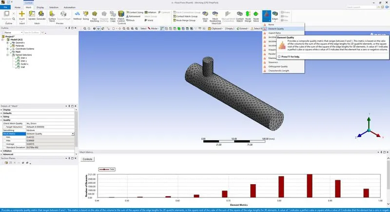
This is an image of the mesh creating for a short T geometry.

The mesh metric gives a good percentage of the mesh quality.

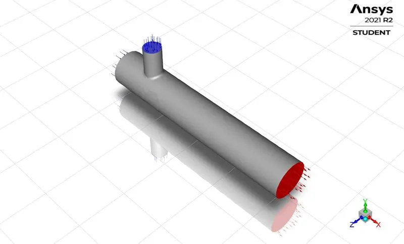
This gives us a 3D view of the same.

Plotting all the details from a short T for a momentum ratio of 2, using the k-epsilon solver.

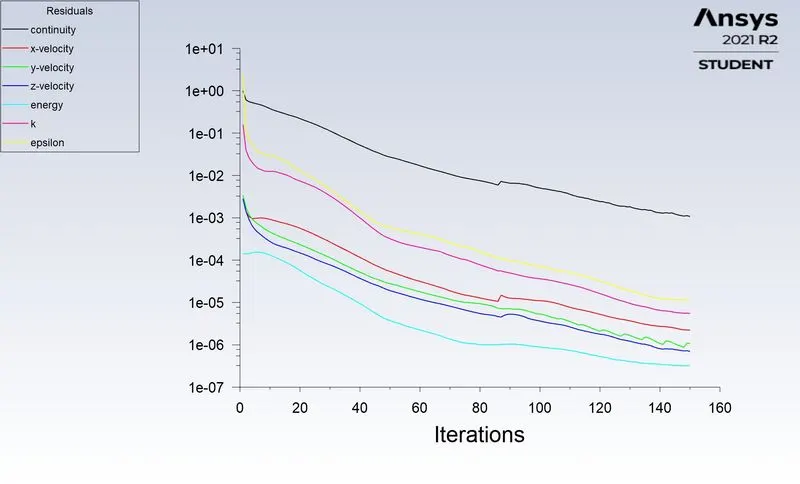
• Scaled Residuals

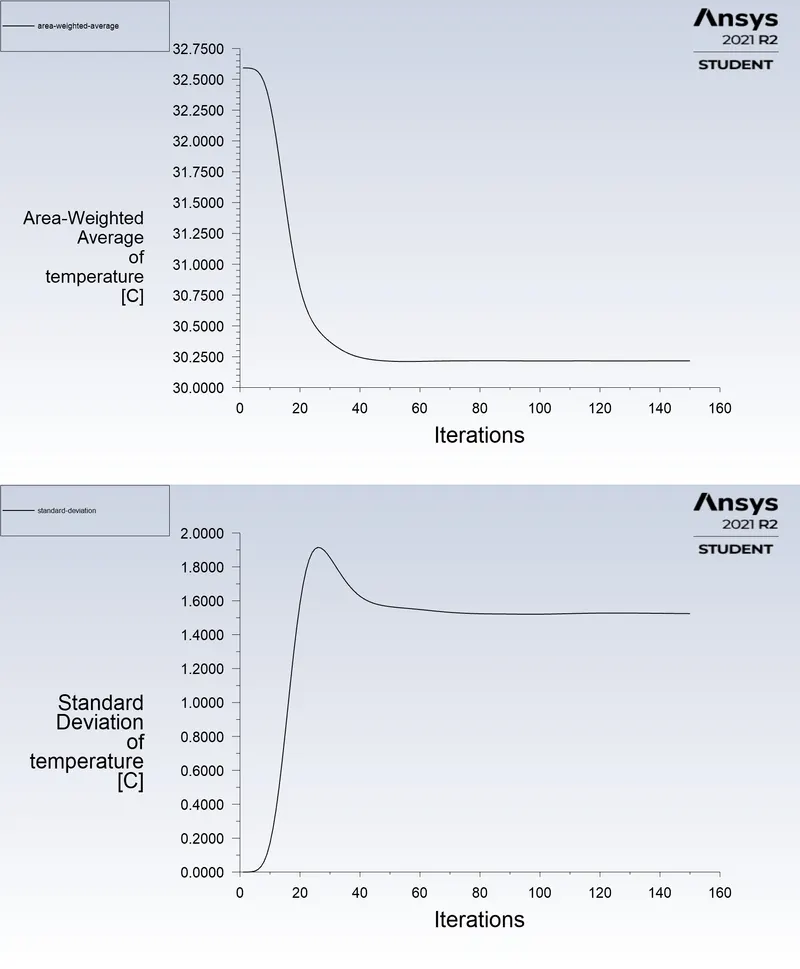
• Area Weighted average and standard deviation of temperature at the outlet.

• Velocity and Temperature contour profile along length of Tee.

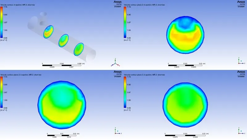
• Velocity contour along cut planes of tee.

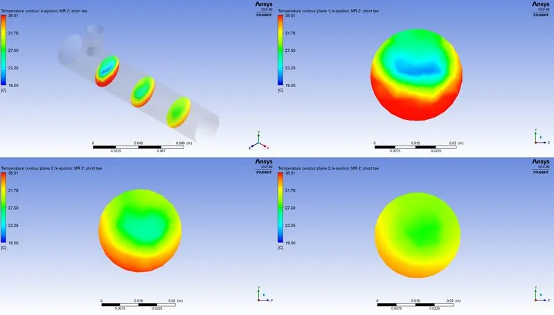
• Temperature contour along cut planes of tee.

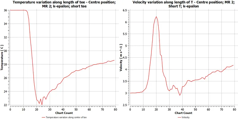
• Temperature and Velocity line plot along length of Tee.

Plotting all the details from a short T for a momentum ratio of 2, using the k-omega SST solver.

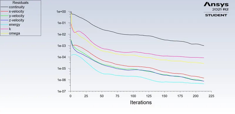
• Scaled Residuals

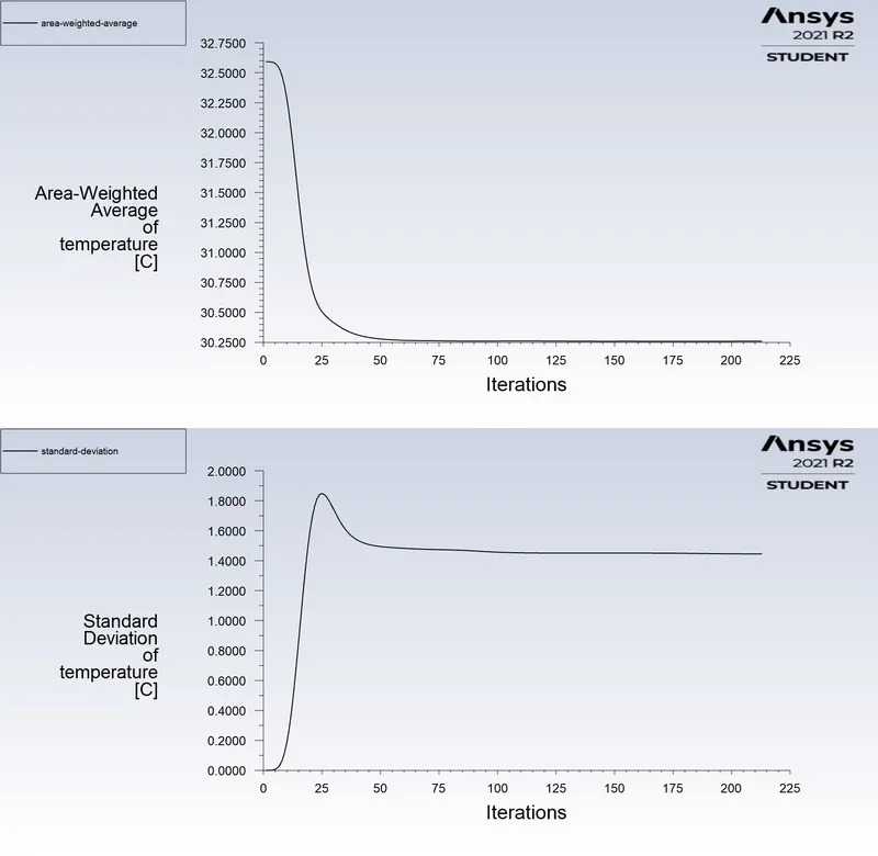
• Area Weighted average and Standard deviation of temperature at outlet.

• Temperature and Velocity contour plots along length of Tee.

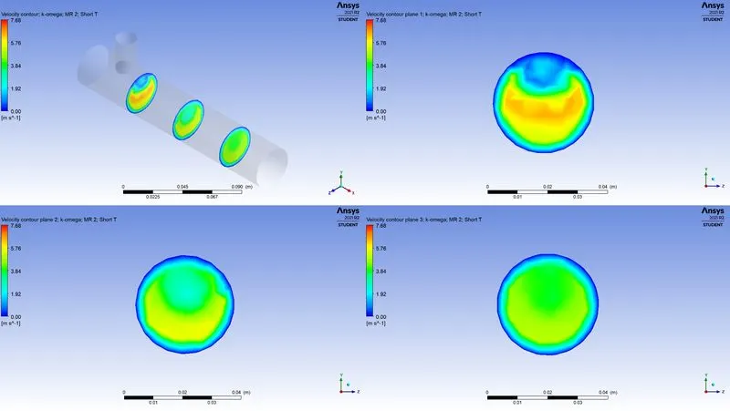
• Velocity contour plot along cut planes of Tee.

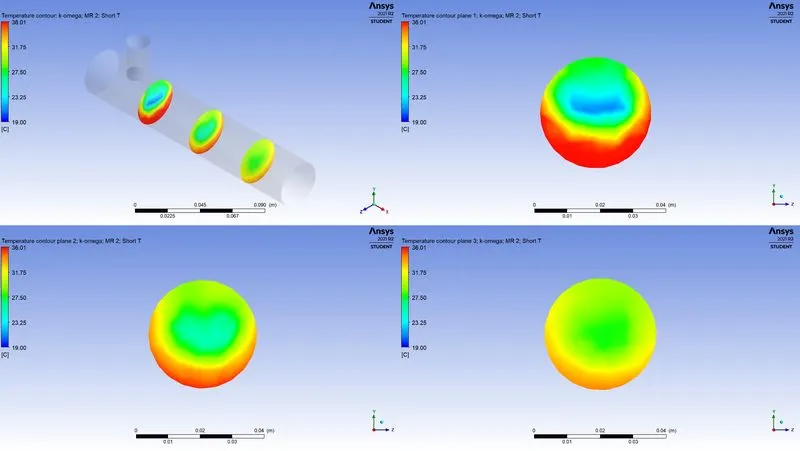
• Temperature contour plot along cut planes of Tee.

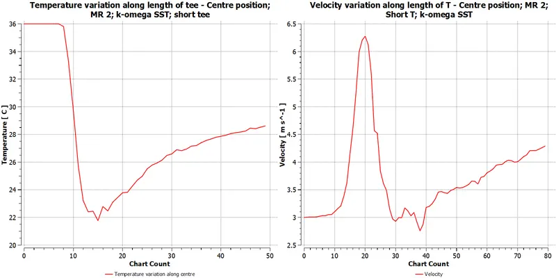
• Temperature and Velocity line plot along length of Tee.

Plotting all the details from a short T for a momentum ratio of 4, using the k-epsilon solver.

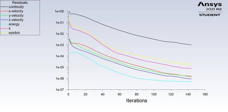
• Scaled Residuals

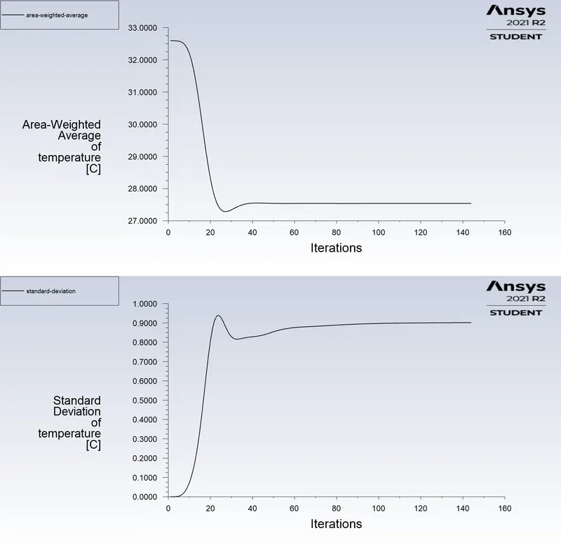
• Area Weighted average and Standard deviation of temperature at outlet.

• Temperature and Velocity contour plots along length of Tee.

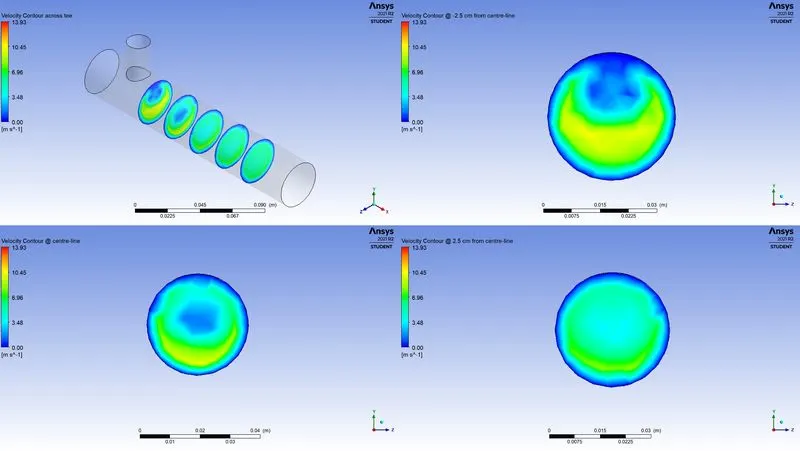
• Velocity contour plots across cut planes of tee - 1

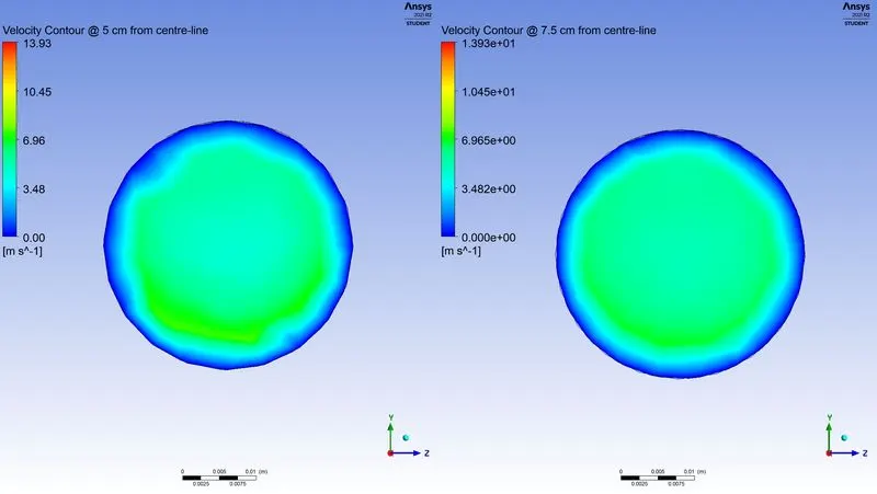
• Velocity contour plots across cut planes of tee - 2

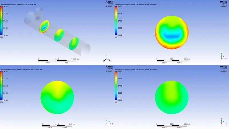
• Temperature contour plots across cut planes of tee

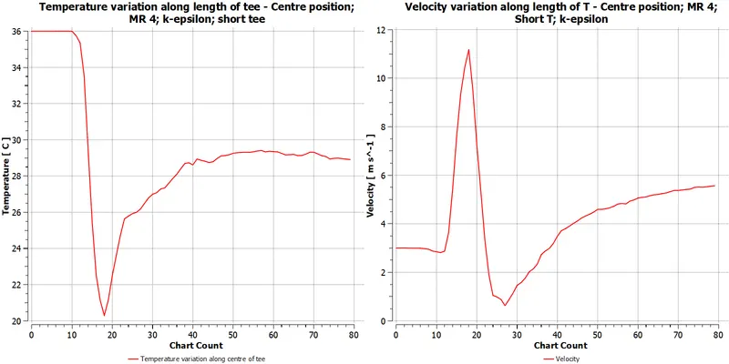
• Temperature and Velocity line plot along length of Tee.

Plotting all the details from a short T for a momentum ratio of 4, using the k-omega SST solver.

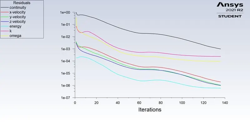
• Scaled Residuals

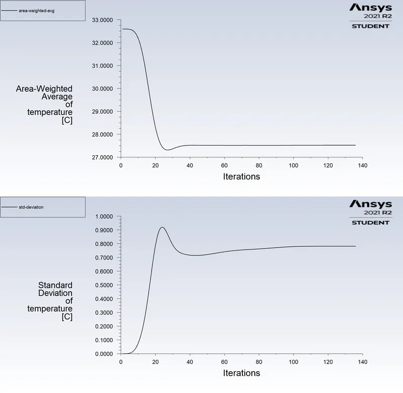
• Area Weighted average and Standard deviation of temperature at outlet.

• Temperature and Velocity contour plots along length of Tee.

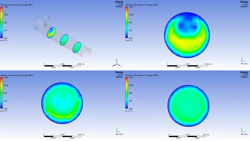
• Velocity contour plot across cut planes of tee.

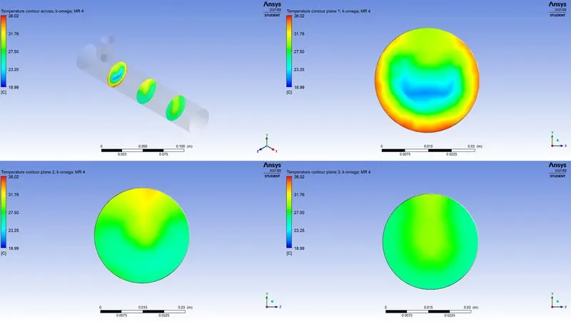
• Temperature contour plot across cut planes of tee.

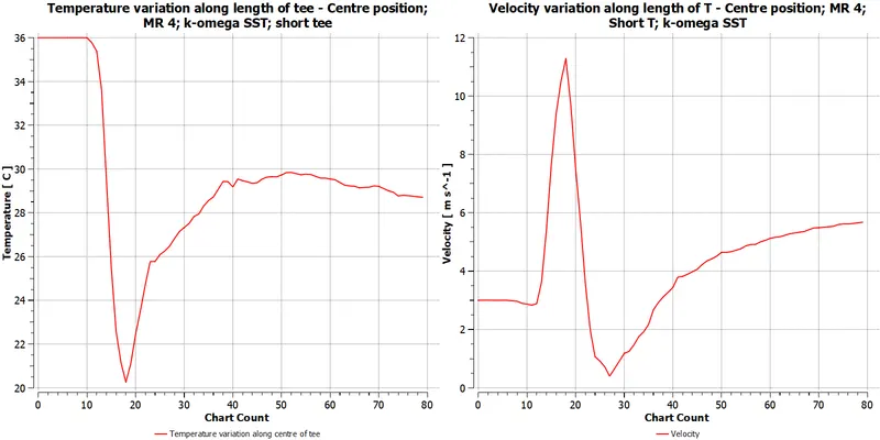
• Temperature and Velocity line plot along length of Tee.

Plotting all the details from a Long T for a momentum ratio of 2, using the k-omega SST solver.

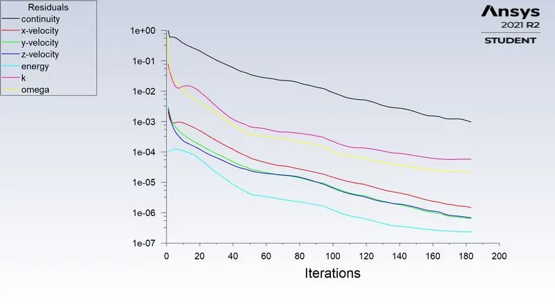
• Scaled Residuals

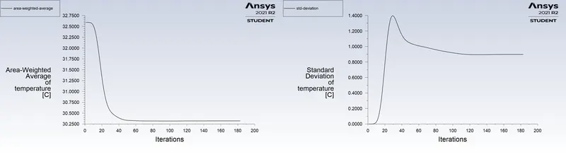
• Area Weighted average and Standard deviation of temperature at outlet.

• Temperature and Velocity contour plots along and across the cut plane length of Tee.

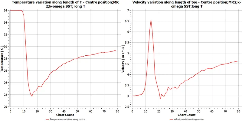
• Temperature and Velocity line plot along length of Tee.

Plotting all the details from a Long T for a momentum ratio of 4, using the k-omega SST solver.

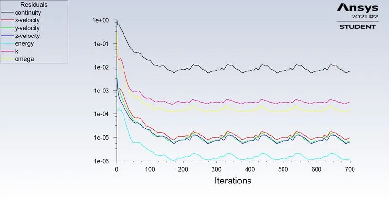
• Scaled Residuals

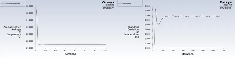
• Area Weighted average and Standard deviation of temperature at outlet.

• Temperature and Velocity contour plots along and across the cut plane length of Tee.

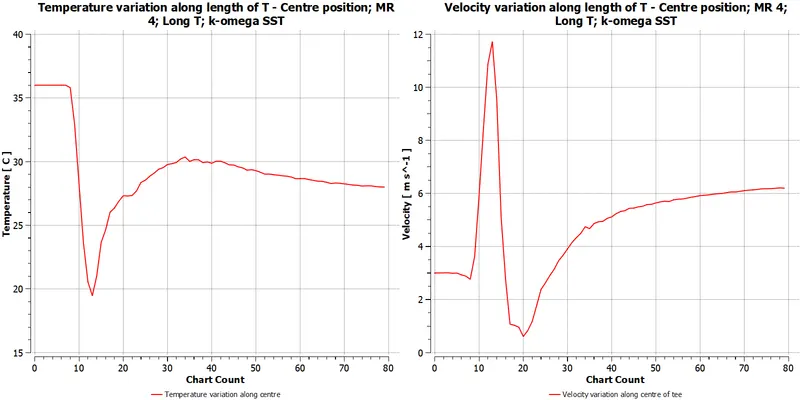
• Temperature and Velocity line plot along length of Tee.

• Comparing various geometries and solvers in a tabulated form.

	Short Tee; MR 2; k-epsilon Realizable	Short Tee; MR 2; k-omega SST	Short Tee; MR 4; k-epsilon Realizable	Short Tee; MR 4; k-omega SST	Long Tee; MR 2; k-omega SST	Long Tee; MR 4; k-omega SST
Cells	12,444	12,444	12,444	12,444	15,282	15,282
Average Outlet Temperature	30.217	30.259	27.539	27.52	30.32	27.487
Number of Iterations to converge	153	212	144	138	183	-
Standard Deviation	1.52	1.45	0.901	0.7813	0.879	0.684

As a side note, the k-omega SST model for a long tee wasn’t able to reach a convergence for as many as 650 iterations at least as the residuals reached an asymptotic value around 150 iterations, this value being higher than the terminating criteria of convergence of the software.

Mesh Independent Study

A very quick mesh independence study has been carried out for a particular case.

In order to validate the mesh independence, we shall consider the short tee geometry, with k-omega SST solver and momentum ratio of 4.

Mesh size (mm)	Number of cells	Iterations to converge	Average Temperature at outlet	Standard deviation of temperature at outlet
10.219	12,444	145	27.528	1.14
4	21,900	141	27.571	1.33
3	39,375	219	27.565	0.91
2	105,058	152	27.55	1.26

The results obtained with different mesh sizes have been tabulated and analysed with the initial default mesh size. Upon analysis of the tabulated values, we find that the mesh convergence has been attained as the resulting solution values do not differ, except mildly, in magnitude.

As a side note, the number of iterations for converge in a mesh size of 3 mm could be more as the mesh quality is affected resulting in an increased number of cells with lower mesh quality. I cannot shed more light on the same, would need to work some more on the same though.

Effect on momentum ratio on results.

Momentum ratio of 2 gives us a velocity double in magnitude for the cold fluid as compared to the hot fluid. Similarly, a momentum ratio of 4 gives us a velocity 4 times in magnitude for the cold fluid as compared to the hot fluid velocity.

From results, we see that cold fluid velocity with a higher magnitude has a better mixing of temperature at the outlet compared to MR 2 case.

Effect of length on results.

Upon changing the length of geometry, we do not see any major differences in the outlet temperature. The secondary diffusion that does takes place along the length of the geometry is negligible and does not affect the temperature at the outlet.

Thus, a short T with a momentum ratio of 4 works just fine.