Week 7 - Simulation of a 1D Super-sonic nozzle flow simulation using Macormack Method
Main Script calling non conservative and conservative functions.
clear all
close all
clc

%% Defining the common parameters

L = 3;
n = [61,31];
gamma = 1.4;
C = 0.5;
nt = 1:1400;

%% The subsonic-supersonic isentropic nozzle solution: Non-Conservation Form

[drho_dt,x,A,rho,V,T_throat,p,M,rho_throat,mfr,p_throat,M_throat] = non_conservation_f(L,n(2),gamma,C,nt);

%% The subsonic-supersonic isentropic nozzle solution: Conservation Form

rho_c_throat_steady = cell(1,numel(n));
T_c_throat_steady = cell(1,numel(n));
p_c_throat_steady = cell(1,numel(n));
M_c_throat_steady = cell(1,numel(n));

for k = 1:length(n)
[x_c,A_c,rho_c,V_c,T_c,mfr_c,U_1,U_2,U_3,dt_c,...
    p_c,M_c,rho_c_old,T_c_old,rho_c_throat,...
    T_c_throat,p_c_throat,M_c_throat,V_c_throat,V_c_old] = conservation_f(C,L,n(k),gamma,nt);

rho_c_throat_steady{k} = rho_c_throat;      % {1} is for 61 nodes {2} for 31.
T_c_throat_steady{k} = T_c_throat;
p_c_throat_steady{k} = p_c_throat;
M_c_throat_steady{k} = M_c_throat;
end

%% Steady state mass flow variation - Conservation vs NonConservation

figure('name','Detailed comparison of steady state mass flow variation')
mfr_exact = 0.579;
plot(x_c,mfr_c)
annotation('textarrow',[0.69 0.6],[0.5 0.31],'String','Conservative form');
hold on
plot(x,mfr)
annotation('textarrow',[0.5 0.64],[0.7 0.5],'String','Non-Conservative form');
plot([0 3],[mfr_exact mfr_exact],'--','linewidth',1.5)
text(1.7,0.581,'Exact Analytical Solution')
xlabel('x/L')
ylabel('Nondimensional mass flow (\rhoVA)/(\rho_0a_0A*)')
title({'Non-Conversation vs Conservation form for ';...
    'steady state mass flow rate'})

%% Comparision of steady state results - Conservation vs NonConservation

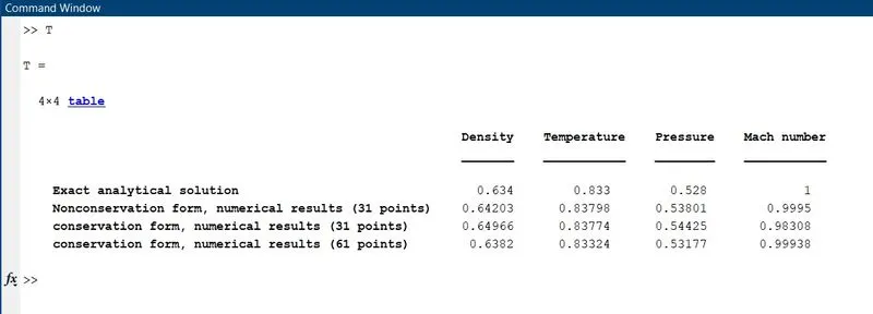
T = table([0.634;rho_throat(1400);rho_c_throat_steady{2}(1400);rho_c_throat_steady{1}(1400)],...
    [0.833;T_throat(1400);T_c_throat_steady{2}(1400);T_c_throat_steady{1}(1400)],...
    [0.528;p_throat(1400);p_c_throat_steady{2}(1400);p_c_throat_steady{1}(1400)],...
    [1.000;M_throat(1400);M_c_throat_steady{2}(1400);M_c_throat_steady{1}(1400)],...
    'VariableNames',{'Density','Temperature','Pressure','Mach number'},...
    'RowNames',{'Exact analytical solution';...
    'Nonconservation form, numerical results (31 points)';...
    'conservation form, numerical results (31 points)';...
    'conservation form, numerical results (61 points)'});

%% Clearing clutter

close figure 1 figure 2 figure 3 figure 5 figure 6 figure 7 figure 8 figure 9
Non-Conservative form function script.
function [drho_dt,x,A,rho,V,T_throat,p,M,rho_throat,mfr,p_throat,M_throat] = non_conservation_f(L,n,gamma,C,nt)


x = linspace(0,L,n);
dx = L/(n-1);

% Initial values rho,T and V
A = 1 + 2.2*((x-1.5).^2);
rho = 1-0.3146*x;
T = 1 - 0.2314*x;
V = (0.1 + 1.09*x).*(T.^0.5);

% Pre-Allocate memory
rho_throat = nan(1,length(nt));
T_throat = nan(1,length(nt));
p_throat = nan(1,length(nt));
M_throat = nan(1,length(nt));
drho_dt = nan(1,n);
dV_dt = nan(1,n);
drho_dt_avg = nan(1,length(nt));
dV_dt_avg = nan(1,length(nt));

% Calculating time step
a = T.^0.5;
dt = (C*dx)./(a+V);
dt = min(dt);

% Grid point corresponding to throat
throat = round(n/2);

%% Time Marching

for j = 1:length(nt)
    % Calculating values for internal points
    for i = 2:n-1

        rho_old = rho;
        T_old = T;
        V_old = V;

        % PREDICTOR STEPS
        dV_dx = (V(i+1) - V(i))./dx;
        dloga_dx = (log(A(i+1)) - log(A(i)))./dx;
        drho_dx = (rho(i+1) - rho(i))./dx;
        dT_dx = (T(i+1) - T(i))./dx;
        % Predictor Derivatives
        drho_dt_p = (-rho(i)*dV_dx)-(rho(i)*V(i)*dloga_dx)-(V(i)*drho_dx);
        dV_dt_p = (-V(i)*dV_dx)-((1/gamma)*(dT_dx+(T(i)/rho(i))*drho_dx));
        dT_dt_p = (-V(i)*dT_dx)-((gamma-1)*T(i)*(dV_dx+(V(i)*dloga_dx)));
        % Barred Variables
        rho(i) = rho(i) + (drho_dt_p*dt);
        V(i) = V(i) + (dV_dt_p*dt);
        T(i) = T(i) + (dT_dt_p*dt);

        % CORRECTOR STEPS
        dV_dx_c = (V(i) - V(i-1))./dx;
        dloga_dx_c = (log(A(i)) - log(A(i-1)))./dx;
        drho_dx_c = (rho(i) - rho(i-1))./dx;
        dT_dx_c = (T(i) - T(i-1))./dx;
        % Corrector Derivatives
        drho_dt_c = (-rho(i)*dV_dx_c)-(rho(i)*V(i)*dloga_dx_c)-(V(i)*drho_dx_c);
        dV_dt_c = (-V(i)*dV_dx_c)-((1/gamma)*(dT_dx_c+(T(i)/rho(i))*drho_dx_c));
        dT_dt_c = (-V(i)*dT_dx_c)-((gamma-1)*T(i)*(dV_dx_c+(V(i)*dloga_dx_c)));

        % AVERAGE DERIVATIVES
        drho_dt(i) = 0.5*((drho_dt_p)+(drho_dt_c));
        dV_dt(i) = 0.5*((dV_dt_p)+(dV_dt_c));
        dT_dt = 0.5*((dT_dt_p)+(dT_dt_c));

        % Final NonDimensional variables at time step
        rho(i) = rho_old(i) + (drho_dt(i)*dt);
        V(i) = V_old(i) + (dV_dt(i)*dt);
        T(i) = T_old(i) + (dT_dt*dt);

    end

        drho_dt_avg(j) = abs(drho_dt(throat));
        dV_dt_avg(j) = abs(dV_dt(throat));

        % Entry Boundary Conditions
        V(1) = 2*V(2)-V(3);

        % Exit Boundary Conditions
        V(n) = 2*V(n-1)-V(n-2);
        rho(n) = 2*rho(n-1)-rho(n-2);
        T(n) = 2*T(n-1)-T(n-2);

        % NonDimensional Pressure
        p = rho.*T;         % pressure
        M = V./(T.^0.5);    % Mach number
        mfr = rho.*A.*V;    % mass flow rate

        % Extract values from throat area
        rho_throat(j) = rho(throat);
        T_throat(j) = T(throat);
        p_throat(j) = p(throat);
        M_throat(j) = M(throat);

%% Plot of Variation of Mass flow rate distribution inside the nozzle at different time steps during the time-marching process

        for h = [1,50,100,150,200,700]
            if h == j
                plot(x,mfr)
                hold on
                grid on
                xlabel('Nondimensional distance through nozzle (x)')
                ylabel('Nondimensional mass flow (\rhoVA)/(\rho_0a_0A*)')
                title({'Instantaneous distributions of the nondimensional';...
                'mass flow as a function of distance through the nozzle';...
                'at six different times during the time-marching';...
                'approach to the steady state'});
            end
        end
end
        legend('1','50','100','150','200','700')
%% Plot of Time-wise variation of primitive variables
% Time wise variation of rho,T,p & M at nozzle throat

figure('name','Time-wise variation of primitive variables - non conservation','windowstate','maximized')

        subplot(221)
        plot(nt,rho_throat)
        xlabel('Number of time steps')
        ylabel('\rho/\rho_0')
        title(sprintf('Timewise variations of Density at nozzle throat at grid point i = %g, where A=1',throat))

        subplot(222)
        plot(nt,T_throat)
        xlabel('Number of time steps')
        ylabel('T/T_0')
        title(sprintf('Timewise variations of Temperature at nozzle throat at grid point i = %g, where A=1',throat))

        subplot(223)
        plot(nt,p_throat)
        xlabel('Number of time steps')
        ylabel('p/p_0')
        title(sprintf('Timewise variations of Pressure at nozzle throat at grid point i = %g, where A=1',throat))

        subplot(224)
        plot(nt,M_throat)
        xlabel('Number of time steps')
        ylabel('M')
        title(sprintf('Timewise variations of Mach number at nozzle throat at grid point i = %g, where A=1',throat))


%% Plot of Steady-state distribution of primitive variables along x

figure('name','steady state values - non-conservative form')
plot(x,rho,'r',x,T,'g',x,V,'b',x,p,'k')
legend('Density','Temperature','Velocity','pressure','location','NorthWest')
grid on
xlabel('Characteristic Length of domain')
ylabel('Primitive variables')
title({'Steady-state distribution of primitive variables along ';...
    'length of nozzle - Non-Conservative form'})


%% Plot for variation of time derivatives

figure('name','Number of time steps vs Residuals')
semilogy(nt,drho_dt_avg)
hold on
semilogy(nt,dV_dt_avg,'linestyle','- -')
xlabel('Number of time steps')
ylabel('Residual')
legend('\fontsize{16}\delta\rho/\deltat','\fontsize{16}\deltaV/\deltat')
title({'Timewise variation of the absolute values of ';...
    'the time derivates of nondimensional density and velocity ';...
    'at the nozzle throat - Nonconservative'})

end
Conservative form function script.
function [x_c,A_c,rho_c,V_c,T_c,mfr_c,U_1,U_2,U_3,dt_c,...
    p_c,M_c,rho_c_old,T_c_old,rho_c_throat,...
    T_c_throat,p_c_throat,M_c_throat,V_c_throat,V_c_old] = conservation_f(C,L,n,gamma,nt)

x_c = linspace(0,L,n);
dx_c = L/(n-1);

% Grid point corresponding to throat
throat = round(n/2);

% Pre-Allocate memory
dU1_dt_p = nan(1,n);
dU2_dt_p = nan(1,n);
dU3_dt_p = nan(1,n);
dU1_dt_c = nan(1,n);
dU2_dt_c = nan(1,n);
dU3_dt_c = nan(1,n);
mfr_store = cell(1,3);

rho_c_throat = nan(1,length(nt));
T_c_throat = nan(1,length(nt));
p_c_throat = nan(1,length(nt));
M_c_throat = nan(1,length(nt));
V_c_throat = nan(1,length(nt));
mfr_c_throat = nan(1,length(nt));

rho_c = nan(1,n);
T_c = nan(1,n);

for i = 1:n
    if x_c(i) <= 0.5           % rho and T
        rho_c(i) = 1;
        T_c(i) = 1;
    elseif (x_c(i) >= 0.5) && (x_c(i) <= 1.5)
        rho_c(i) = 1 - 0.366*(x_c(i)-0.5);
        T_c(i) = 1 - 0.167*(x_c(i)-0.5);
    elseif x_c(i) > 1.5 && x_c(i) <= 3
        rho_c(i) = 0.634 - 0.3879*(x_c(i)-1.5);
        T_c(i) = 0.833 - 0.3507*(x_c(i)-1.5);
    end
end

% Initial values of the primitives
A_c = 1 + 2.2*((x_c-1.5).^2);       % Area
V_c = 0.59./(rho_c.*A_c);           % Velocity
rho_c_old = rho_c;
T_c_old = T_c;
V_c_old = V_c;

% Initial conditions
U_1 = rho_c.*A_c;
U_2 = 0.59*ones(1,n);
U_3 = (U_1).*((T_c/(gamma-1))+((gamma/2)*(V_c.^2)));

for j = 1:length(nt)

    % Storing initial values
    U_1_old = U_1;
    U_2_old = U_2;
    U_3_old = U_3;

    % Calculating the minimum delta t
    a = T_c.^0.5;
    dt_c = (C*dx_c)./(a+V_c);
    dt_c = min(dt_c);

    for i = 2:n-1

        % Flux vectors
        F_1 = U_2;
        fterm = (((U_2).^2)./U_1);
        F_2 = fterm + (((gamma-1)/gamma)*(U_3-((gamma/2)*fterm)));
        term1 = (U_2.*U_3)./U_1;
        term2 = U_2.^3./U_1.^2;
        F_3 = (gamma*term1)-((gamma*(gamma-1)/2)*term2);

        % Source term upgrade
        J_2 = (1/gamma)*rho_c(i)*T_c(i)*((A_c(i+1)-A_c(i))/dx_c);

        % Predictor steps
        dU1_dt_p(i) = -(F_1(i+1)-F_1(i))/dx_c;
        dU2_dt_p(i) = -((F_2(i+1)-F_2(i))/dx_c) + J_2;
        dU3_dt_p(i) = -(F_3(i+1)-F_3(i))/dx_c;

        % Updating Solution vectors - U bar
        U_1(i) = U_1(i) + (dU1_dt_p(i))*dt_c;
        U_2(i) = U_2(i) + (dU2_dt_p(i))*dt_c;
        U_3(i) = U_3(i) + (dU3_dt_p(i))*dt_c;

    end

    U_2(1) = 2*U_2(2)-U_2(3);
    V_c(1) = U_2(1)/U_1(1);
    U_3(1) = U_1(1)*((T_c(1)/(gamma-1))+((gamma/2)*(V_c(1)^2)));

    % Updating Flux terms - barred
    F_1 = U_2;
    fterm = (((U_2).^2)./U_1);
    F_2 = fterm + (((gamma-1)/gamma)*(U_3-((gamma/2)*fterm)));
    term1 = (U_2.*U_3)./U_1;
    term2 = U_2.^3./U_1.^2;
    F_3 = (gamma*term1)-((gamma*(gamma-1)/2)*term2);

    % Update the primitives - barred
    rho_c = U_1./A_c;
    T_c = (gamma-1)*((U_3./U_1)-((gamma/2)*((U_2./U_1).^2)));
    V_c = U_2./U_1;


    for i = 2:n-1
        % Source term - Corrector Step
        J_2_c = (1/gamma)*rho_c(i)*T_c(i)*((A_c(i)-A_c(i-1))/dx_c);

        % Corrector Steps
        dU1_dt_c(i) = -(F_1(i)-F_1(i-1))/dx_c;
        dU2_dt_c(i) = -((F_2(i)-F_2(i-1))/dx_c)+ J_2_c;
        dU3_dt_c(i) = -(F_3(i)-F_3(i-1))/dx_c;

        % Average derivatives
        dU1_dt = 0.5*(dU1_dt_p + dU1_dt_c);
        dU2_dt = 0.5*(dU2_dt_p + dU2_dt_c);
        dU3_dt = 0.5*(dU3_dt_p + dU3_dt_c);

        % Final update of Solution vector elements,U
        U_1(i) = U_1_old(i) + (dU1_dt(i))*dt_c;
        U_2(i) = U_2_old(i) + (dU2_dt(i))*dt_c;
        U_3(i) = U_3_old(i) + (dU3_dt(i))*dt_c;

    end

    % Inlet boundary
    rho_c(1) = 1;
    T_c = 1;
    U_1(1) = rho_c(1)*A_c(1);
    U_2(1) = 2*U_2(2) - U_2(3);
    V_c(1) = U_2(1)/U_1(1);
    U_3(1) = U_1(1)*(T_c(1)/(gamma-1))+((gamma/2)*V_c(1)^2);

    % Exit boundary
    U_1(n) = 2*U_1(n-1) - U_1(n-2);
    U_2(n) = 2*U_2(n-1) - U_2(n-2);
    U_3(n) = 2*U_3(n-1) - U_3(n-2);

    % Final update of primitives
    rho_c = U_1./A_c;
    V_c = U_2./U_1;
    T_c = (gamma-1)*((U_3./U_1)-((gamma/2)*(V_c.^2)));
    p_c = rho_c.*T_c;
    M_c = V_c./(T_c.^0.5);
    mfr_c = U_2;

    % Extract values from throat area
    rho_c_throat(j) = rho_c(throat);
    T_c_throat(j) = T_c(throat);
    p_c_throat(j) = p_c(throat);
    M_c_throat(j) = M_c(throat);
    V_c_throat(j) = V_c(throat);
    mfr_c_throat(j) = mfr_c(throat);

    % This is to plot mass flow rate at specific time steps
    if j == 100
        mfr_store{1} = mfr_c;
    elseif j == 200
        mfr_store{2} = mfr_c;
    elseif j == 700
        mfr_store{3} = mfr_c;
    end

end

%% Plot of Variation of Mass flow rate distribution inside the nozzle at different time steps during the time-marching process

if n == 31

    figure('name','mass flow rate for 31 grid points - Conservative form')

    plot(x_c,mfr_store{1},x_c,mfr_store{2},x_c,mfr_store{3})
    grid on
    xlabel('Nondimensional distance through nozzle (x)')
    ylabel('Nondimensional mass flow (\rhoVA)/(\rho_0a_0A*)')
    title({'Instantaneous distributions of the nondimensional';...
        'mass flow as a function of distance through the nozzle';...
        'at 3 different times during the time-marching';...
        'approach to the steady state'});
    legend('100','200','700')

end

if n == 61

    figure('name','mass flow rate for 61 grid points - Conservative form')

    plot(x_c,mfr_store{1},x_c,mfr_store{2},x_c,mfr_store{3})
    grid on
    xlabel('Nondimensional distance through nozzle (x)')
    ylabel('Nondimensional mass flow (\rhoVA)/(\rho_0a_0A*)')
    title({'Instantaneous distributions of the nondimensional';...
        'mass flow as a function of distance through the nozzle';...
        'at 3 different times during the time-marching';...
        'approach to the steady state'});
    legend('100','200','700')

end

%% Plot of Time-wise variation of primitive variables at throat
if n == 31

    figure('name','Variation of primitives at throat - 31 grid points')
    plot(nt,rho_c_throat,'linewidth',1.5)
    hold on
    plot(nt,T_c_throat,'linewidth',1.5)
    plot(nt,p_c_throat,'linewidth',1.5)
    plot(nt,M_c_throat,'linewidth',1.5)
    plot(nt,V_c_throat,'linewidth',1.5)
    plot(nt,mfr_c_throat,'linewidth',1.5)
    xlabel('Time steps(nt)')
    ylabel('Non dimensional Parameters')
    title({'Conservation form - Time-Wise Variation of Primitive ';...
        'variables at throat for 31 grid points'})
    legend('Density - \rho','Temperature','Pressure','Mach number','Velocity','mass flow rate')
    grid on
    hold off

elseif n == 61

    figure('name','Variation of primitives at throat - 61 grid points')
    plot(nt,rho_c_throat,'linewidth',1.5)
    hold on
    plot(nt,T_c_throat,'linewidth',1.5)
    plot(nt,p_c_throat,'linewidth',1.5)
    plot(nt,M_c_throat,'linewidth',1.5)
    plot(nt,V_c_throat,'linewidth',1.5)
    plot(nt,mfr_c_throat,'linewidth',1.5)
    xlabel('Time steps(nt)')
    ylabel('Non dimensional Parameters')
    title({'Conservation form - Time-Wise Variation of Primitive ';...
        'variables at throat for 61 grid points'})
    legend('Density - \rho','Temperature','Pressure','Mach number','Velocity','mass flow rate')
    grid on
    hold off

end
end
Report.
CFD SOLUTION OF SUBSONIC-SUPERSONIC ISENTROPIC NOZZLE FLOW: MACCORMACK’S TECHNIQUE
We shall be applying MacCormack’s technique to the discretized form of the conservation and non-conservation form of governing partial differential equations. In order to do so, we first understand MacCormack’s technique.
UNDERSTANDING MACCORMACK’S TECHNIQUE
MacCormack’s technique is a variant of the Lax-Wendorff approach.
It is an explicit finite-difference technique which is second order accurate in both space and time.
Using Taylor series expansion about the next time step, we get a first order derivative of the property which we shall call as the average partial time derivative. This shall be discretized using the predictor and corrector step.
In predictor step, we replace spacial derivatives of the equation with forward differences to calculate the first order derivatives. Following which, we expand the properties using Taylor series with the derivative calculated above. We call these properties as barred properties.
Corrector Step: In this step, we substitute the barred values in the discretized equation for the partial derivatives, only this time, we use a backward difference scheme to the spacial terms.
The average time derivative we obtain is by calculating the average of the derivates calculated from above.
THE SETUP
Governing flow equations shall be couched into PDE’s for time marching solution.
The finite-difference expressions pertaining to MacCormack’s technique will be set up
Other details as calculation of time step and boundary conditions shall be formulated.
GOVERNING FLOW EQUATIONS
The integral form of the continuity equation is given as
`∂/(∂t) ∭_VρdV+∬_SρV⋅dS=0`
Rearranging terms and with mathematical manipulations, we arrive at the partial differential equation form of the continuity equation.
`(∂(ρA))/(∂t)+(∂(ρAV))/(∂x)=0`
Similarly, writing momentum equation for quasi-one-dimensional flow, in the non-conservation form, we have,
`ρ (∂v)/(∂t)+ρV (∂V)/(∂x)=-(∂p)/(∂x)`
Non-conservation form of the energy equation expressed in terms of internal energy, appropriate to unsteady, quasi-one-dimensional flow.
`ρ(∂e)/(∂t)+ρV (∂e)/(∂x)=-P (∂V)/(∂x)-pV (∂(lnA))/(∂x)`
Writing all the above equations in nondimensional form, we get,
Continuity:
`(∂ρ^')/(∂t^' )=-ρ (dV')/(∂x^' )-ρ^' v^' (∂(lnA^' ) )/(∂x^' )-V^' (∂ρ^')/(∂x^' )`
Momentum:
`(∂V^')/(∂t^' )=-V^' (∂v^')/(∂x^' )-1/γ ((∂T^')/(∂x^' )+T^'/ρ^' (∂ρ^')/(∂x^' ))`
Energy:
`(∂T^')/(∂t^' )=-v^' (∂T^')/(∂x^' )-(γ-1) T^' [(∂v^')/(∂x^' )+v^' (∂(lnA^' ) )/(∂x^' )]`
CALCULATION OF TIME STEP
The governing equations we are dealing with are hyperbolic with respect to time.
Magnitude of time step is calculated using the formula
`Δt=C(Δx)/(a+V)`
C is the courant number.
C<1 for an explicit scheme to be stable.
We calculate time step at all the internal grid points and chose the minimum value from all of these.
BOUNDARY CONDITIONS
The inlet to the nozzle is called the inflow boundary and the exit of the nozzle is called the outflow boundary corresponding to point N.
The flow velocity at point 1 is subsonic in nature and at exit is supersonic in nature.
The method of characteristics tells us that at a boundary where one characteristic propagates into the domain, then the value of one dependent flow field variable must be specified at that boundary, and if one characteristic line propagates out of the domain, the value of flow field variable must be allowed to float that that boundary, i.e., it must be calculated in steps of time as a function of the timewise solution of the flow field.
Subsonic inflow boundary.
Based on the above assumptions, we arrive at the formula
`V_1=2V_2-V_3`
Density and temperature are both 1, fixed, independent of time.
Supersonic outflow boundary.
Here, all the variables are allowed to float as all the characteristics move out of the domain.
For the nondimensional variables, we have,
`V_N=2V_(N-1)-V_(N-2)`
`ρ_N=2ρ_(N-1)-ρ_(N-2)`
`T_N=2T_(N-1)-T_(N-2)`
The nozzle shape is specified and held fixed, independent of time. For this case, we take the parabolic area as defined in the book by Anderson.
`A=1+2.2(x-1.5)^2`
At x = 1.5, we have the nozzle throat, a convergent section at x<1.5 and a divergent section at x>1.5.
In order to start the time marching calculations, we must stipulate the initial conditions for the variables given above as a function of x.
Theoretically, these initial conditions can be purely arbitrary but one should choose them in such a way that convergence is reached faster, this of course can be achieved if the initial conditions are chosen as close to steady state as possible.
Choosing the variable density, temperature and velocity.
`ρ=1-0.3146x`
`T=1-0.2314x`
`v=(0.1+1.09x) T^0.5`
The first step is to feed nozzle shape and initial conditions into the program.
Next is to put these initial conditions to initiate calculations pertaining to the predictor step.
Then the predicted values (also known as the barred quantities) are calculated for this, minimum value of time step is calculated as discussed earlier.
In calculation of minimum time step, we have taken a value of courant number of 0.5 and in non-dimensional terms, the speed of sound is taken as square root of temperature.
We now insert the barred quantities to get the values using formulas as discussed under the corrector steps.
The average of the time derivatives is now calculated which completes the corrector step.
Flow field variables at the boundary points are yet to be calculated. This can be done using the formula shown above for V at grid point 1.
Similarly, flow field variables at nozzle exit are calculated.
CONSERVATION FORM
Basic equations used in conservation form
Continuity equation
`(∂(ρA))/(∂t)+(∂(ρAV))/(∂x)=0`
Momentum equation
`(∂(ρA))/(∂t)+(∂[ρAv^2+(1⁄γ)PA])/(∂x)=1/γ p (∂A)/(∂x)`
Energy equation
`(∂[ρ(e/(γ-1)+γ/2 V^2 )A])/(∂t)+(∂[ρ(e/(γ-1)+(γV^2)/2)VA+pAV])/(∂x)=0`
`U_1=ρA`
`U_2=ρAV`
`U_3=ρA(e/(γ-1)+γ/2 V^2 )`
`F_1=ρAV`
`F_2=ρAV^2+1/γ PA`
`F_3=ρAV(e/(γ-1)+γ/2 V^2 )+pAV`
`J_2=1/γ P (∂A)/(∂x)`
With these elements, the equations above can be written as
`(∂U_1)/(∂t)=-(∂F_1)/(∂x)`
`(∂U_2)/(∂t)=-(∂F_2)/(∂x)+J_2`
`(∂U_3)/(∂t)=-(∂F_3)/(∂x)`
These are the equations we wish to solve numerically using MacCormack’s technique.
- The dependent variables, in conservation form, are not primitive variables.
- From the above equations, the numerical solution will give us numbers directly in form of U1 U2 and U3.
- Thus, U is called our solution vector.
- Primitive variables are decoded from these solution vectors.
`ρ=U_1/A`
`V=U_2/U_1`
`T=e=(γ-1)(U_3/U_2 -γ/2 V^2 )`
`p=ρT`
Note:
`e^1=e/e_0 =(c_v T)/(c_v T_0 )=T/T_0 =T^'`
All the primitives in above equations are non-dimensional.
- After obtaining U1, U2 and U3 at each time step, we immediately calculate primitives at that time step from U values.
- Flux vectors, F1, F2 and F3 are taken in terms of solution vectors and not in terms of primitives in the program, as it has been observed that taking F in terms of primitives leads to instabilities causing the solution to blow up after a couple of time steps.
- Thus, F is taken in terms of U by some mathematical rearrangements which leads us to the following relations
F1 = U2
`F_2=(U_2^2)/U_1 +(γ-1)/(γ) [U_3-γ/2 (U_2^2)/U_1 ]`
`F_3=γ (U_2 U_3)/U_1 -(γ(γ-1))/2 (U_2^3)/(U_1^2 )`
`J_2=(γ-1)/γ [U_3-γ/2 (U_2^2)/U_1 ] (∂[lnA ])/(∂x)`
Note:
- The above equations are termed as the pure form of flux terms.
- When primitives, which are decoded from the solution vector, are used to reconstruct flux terms, numerical difficulties usually arise.
- This could be connected to the fact that dependent variables which appear explicitly in above equations are in solution vector forms, not primitive variables. For this reason, it is best to couch flux terms directly in terms of solution vectors.
- The source vector, J2, is taken in terms of primitives and not in solution vector form for ease of programming, even though it contradicts the above points, it is found out that it does not affect the solution.
BOUNDARY CONDITIONS.
- At the subsonic inflow boundary, 2 properties are held fixed and one is allowed to float as discussed previously.
- At the supersonic outflow boundary, all properties are allowed to float.
- Density and temperature are held fixed at inlet. Velocity is allowed to float.
- By holding density fixed, U1 becomes fixed, independent of time.
- Floating value “V” is calculated at the end of each time step by linearly extrapolating the value of U2 from internal grid points.
- Since velocity at grid point 1 is floating, so does U3 as it contains velocity term.
- U1, U2 and U3 at the first grid point at used to calculate flux terms.
- These values of flux terms at inflow boundary are needed to form the rearward differences during corrector steps of MacCormack’s technique.
- Flow properties at the supersonic outflow boundary are obtained by linear interpolation from two adjacent internal grid points.
- Flux terms are calculated from solution vectors and are used to form forward differences during predictor step of MacCormack’s technique.
INITIAL CONDITIONS
- We need initial conditions for solution vectors to start calculations.
- This yields flux terms, which, in turn, will be used to form x-derivates on the right-hand side of the equations at the first-time step.
- Initial conditions for solution vectors are synthesized by assuming the following variations of flow variables.
- Density and temperature are equal to 1. Were x lies between 0 and 0.5.
- When x lies between 0.5 and 1.5, we use the relation,
`ρ=1-0.366(x-0.5)`
`T=1-0.167(x-0.5)`
- When x lies between 1.5 and 3, we use the relation,
`ρ=0.634-0.3879(x-1.5)`
`T=0.833-0⋅3507(x-1.5)`
- These variations are slightly more realistic as compared to the primitives assumed for the initial conditions in non-conservation form solution. This is due to the fact that stability behaviour of the finite difference formulation using the conservation form of the governing equations are slightly more sensitive and therefore we try and start with a more realistic initial condition.
- The initial condition for the variation of velocity: Upon closer inspection we realize that U2 which is one of the dependent variables, is physically the local mass flow, i.e.,
U2 = `rho`AV.
Therefore, for the initial conditions only, we assume ma constant mass flow through the nozzle as 0.59 which is derived from the analytical results and calculate velocity using the below formula.
`V=0.59/(ρA)`
- Finally, initial conditions are obtained as
`U_1=ρA`
`U_2=ρAV`
`U_3=ρA[e/(γ-1)+γ/2 V^2 ]`
TIME STEP CALCULATION
We use the same approach as discussed in the non-conservation form topic. The only difference being that the size of time step will change for each time step as it depends on velocity and velocity, in turn, is a function of x.
EXPLANATION OF THE CODE
- Take U2 from analytical results.
- Take U1 as `ρA`
- U3 is calculated using formula shown in the report.
- Start the time marching loop.
- Assign solution vectors to other variables, this will help in Taylor series expansion to calculate final solution vectors in that time step.
- Calculate time step size using formula as discussed in report.
- Within the internal grid points loop, calculate flux vectors.
- Calculate source terms.
- Execute the predictor step, using forward difference scheme.
- Calculate barred values and end loop.
- Calculate solution vector element at first position, this will help during corrector step which will employ flux term 1 using backward difference scheme.
- Finally, update primitives.
Explaining the plots:
Figure 1
This figure shows the variation of non-dimensional mass flow rate along the nozzle at different time steps when reaching steady state for a non-conservational form of solution.
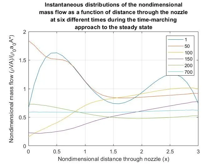
Figure 2
This figure plots the timewise variation of primitive flow field variables, density, pressure, temperature and Mach number at the nozzle throat till steady state – non conservation form
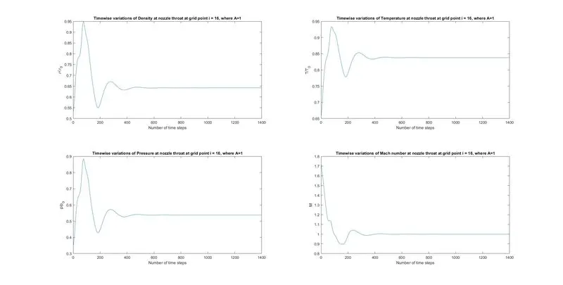
Figure 3
This plot shows how the primitive variables vary along the nozzle on attaining the steady state – non conservation form.
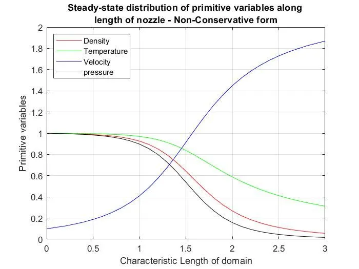
Figure 4
This figure plots how the magnitude of the average derivative of primitive variables pressure and velocity falls with increasing number of time steps. The y-axis is on a logarithmic scale to magnify the amount by which magnitude falls.
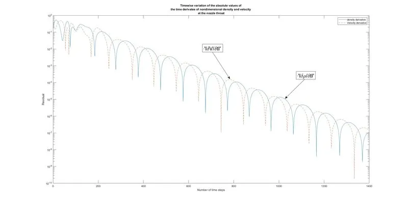
Figure 5
This plot shows the instantaneous distribution of the non-dimensional mass flow rate as a function of distance through the nozzle at three different times during time marching approach for 61 grid points.
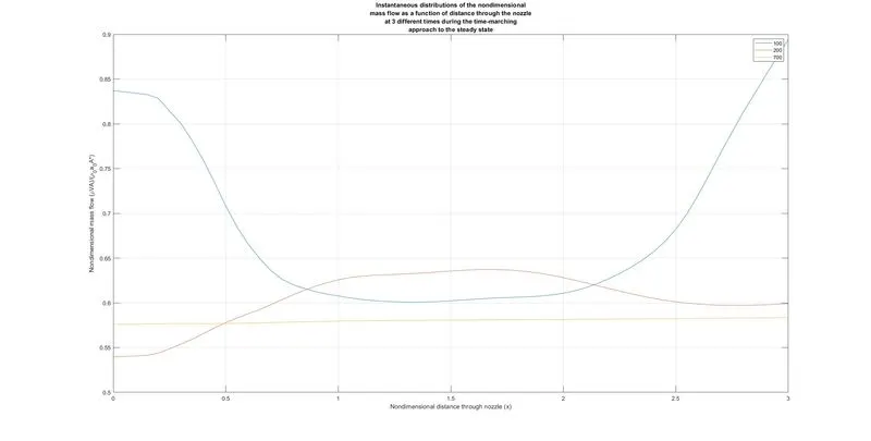
Figure 6
Plot for time wise variation of primitive variable at throat section when programmed with 61 grid points.
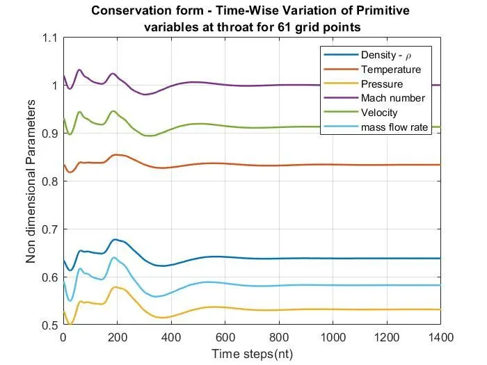
Figure 7
Plot showing variation of the non-dimensional mass flow rate through the nozzle at three different times while approaching steady state and having 31 grid points using conservative form of governing equation.
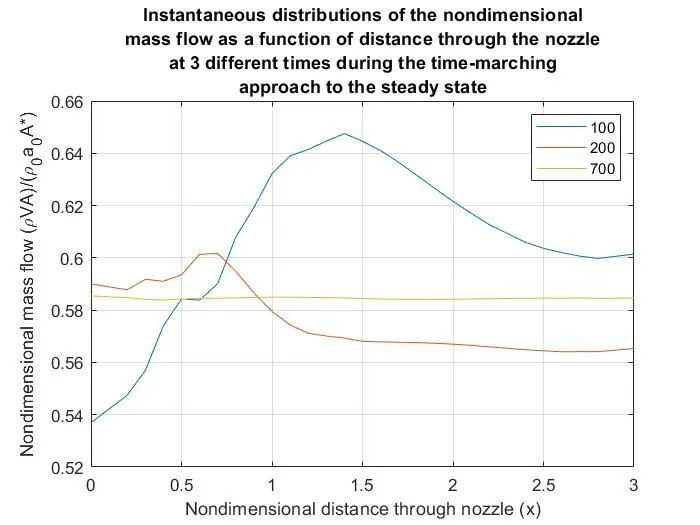
Figure 8
Plot for time wise variation of primitive variable at throat section when programmed with 31 grid points.
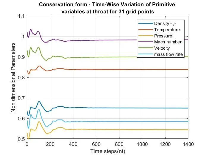
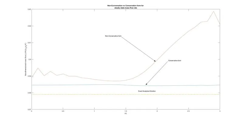
Figure 9
This figure shows the plot of mass flow rate when calculated using conservative form and non-conservative form. It also shows the value obtained using the exact analytical solution.
- Showing the table from the program output.