Week 9 - FVM Literature Review

Finite Volume Method: A Literature Review

The finite volume method (FVM) is a discretization technique for partial differential equations, especially those that arise from physical conservation laws. FVM uses a volume integral formulation of the problem with a finite partitioning set of volumes to discretize the equations.

Before we delve into the interpolation schemes, flux limiters and one-dimensional linear heat conduction, let us start with the General Scalar transport equation and derive 1D diffusion equation.

The General scalar transport equation can be written as,

`(∂(ρϕ))/(∂t)+∇⋅(ρϕu ⃗ )=∇⋅(Γ∇ϕ)+S_ϕ`

Were,

Term 1 = Transient term which is the rate of increase of in the fluid element.

Term 2 = Convective term, which is the net rate of flow of out of the fluid element.

Term 3 = Diffusion term, which is net rate of increase of in diffusion.

Term 4 = Source term.

This is the most generic form of partial differential equation; from which is derived the continuity, momentum and energy equation.

The main or Key step in Finite Volume Method is the integration of the General Scalar Transport Equation on a control Volume.

Before we start with actual integration, we need to understand Gauss-Divergence theorem.

This theorem is used to convert the control integral into surface integrals, as shown below.

`∭_(CV)∇⋅(a ⃗ )dV=∬_(CS)a ⃗n ̂dS`

Why do we need to invoke Gauss-Divergence?

Reason:

`∂/(∂t) ∫_(CV)(ρϕ)dV+∫_(CS)(pϕu ⃗ )⋅n ̂dS=∫_(CS)(Γ∇ϕ)⋅n ̂dS+∫_(CV)S_ϕ dV`

As can be seen from the formula above, we need to have a control surface too in the equation to have a connection between neighbours.

We usually use non-conservative form in the context of Finite Difference Method. Because FDM does not involve integration on a particular Control Volume. So, gauss-Divergence theorem is never invoked. As a result, FDM would not result in a statement of conservation on a cell-by-cell basis, but FDM satisfies the principle of conservation on the entire domain chosen.

In Finite Volume Method, it is satisfied on a cell-by-cell basis.

• Discretization of the equations using Finite Difference methods.

To understand the process of discretization, let us consider a 1D diffusion equation with source term on a uniform mesh.

`Γ (∂^2 ϕ)/(∂x^2 )+S_ϕ=0`

We know the second order derivative using central differencing is given as

`(∂^2 ϕ)/(∂x^2 )=(ϕ_(i+1)-2ϕ_i+ϕ_(i-1))/(Δx^2 )+{0(Δx^2 )}`

Were in the above equation has a truncation error of order of delta x square.

Thus, the above equation becomes

`Γ (∂^2 ϕ)/(∂x^2 )|_i+S_(ϕ_i )=Γ((ϕ_(i+1)-2ϕ_i+ϕ_(i-1))/(Δx^2 ))+S_(ϕ_i )=0`

`((2Γ)/(Δx^2 )) ϕ_i=(Γ/(Δx^2 )) ϕ_(i+1)+(Γ/(Δx^2 )) ϕ_(i-1)+S_(ϕ_i )`

This is the discretized equation we get using FDM.

We obtain a set of algebraic equations.

• Discretization of the equations using Finite Volume methods.

Again, consider 1D diffusion equation as follows,

`d/dx (Γ (dϕ)/(dx))+S_ϕ=0`

Notice in FDM, we have a second order derivative, this is not the case in FVM. Here, we will work with only conservative form, hence, the above form of equation is written.

Integrate the governing equation on a control volume.

`∫_(CV)d/dx (Γ (dϕ)/dx)dV+∫_(CV)S_ϕ dV=0`

This is a definite integral, thus 0 on RHS remains 0.

`∫_(CV)∇⋅(iΓ (dϕ)/dx)dV+∫_(CV)S_ϕ dV=0`

`∫_(CS)iΓ (dϕ)/(dx)dA ⃗ +∫_(CV)S_ϕ dV=0`

`∑_(f=e,w)(iΓ dϕ/dx) (A ⃗_f ) +∫_(CV)S_ϕ dV=0`

`A_e=i ⃗;A_w=-i ⃗`

`iΓ(dϕ)/(dx)+ iΓ (dϕ)/(dx)|_w (-i)+(S_ϕ ) ̅Δv=0`

`(Γ (dϕ)/dx)_e-(Γ (dϕ)/dx)_w+Sϕ ̅Δx=0`

Profile assumption for `ϕ`

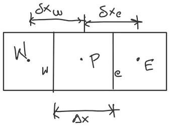
`ϕ` varies linearly between the primary P cell centroid and east cell centroid, E and P and west cell centroid W.

We know the values of `phi` in the cell centroid and need to interpolate them onto the faces joining the cells. Here, we are assuming a linear profile assumption.

`Γ(dϕ)/(dx)|_e=Γ_e (dϕ)/dx|_e=Γ_e ((ϕ_E-ϕ_P)/(δx_e ))`

`Γ ((dϕ)/dx)|_w=Γ_w((ϕ_P-ϕ_w)/(δx_w ))`

`ϕ_E,ϕ_P and ϕ_W` are at the cell centroid.

`Γ_e ((ϕ_E-ϕ_P)/(δx_e ))+Γ_w ((ϕ_P-ϕ_w)/(δx_w ))+(S_ϕ ) ̅Δx=0`

Rearranging and collecting the terms

`(Γ_e/(δx_e )+Γ_w/(δx_w )) ϕ_P=(Γ_e/(δx_e )) ϕ_E+(Γ_w/(δx_w )) ϕ_W`

`a_p ϕ_P=a_E ϕ_E+a_W ϕ_W+S_ϕ Δx`

This is the discretized equation of the general scalar transport equation derived from the finite control volume method.

Interpolation techniques for `Γ_e, Γ_` their advantages and dis-advantages shall be discussed in ensuing topics.

Comments and Conclusion:

1. This discretized equation can be derived for every cell in the domain.
2. The entire process had started off with the statement of conservation – thus, the solution obtained using FVM is always conservative in nature.
3. No matter how coarse the mesh is, the final `ϕ` obtained will satisfy conservation.
4. However, `ϕ` may not be accurate. In order to obtain accurate `ϕ` , a sufficiently small mesh needs to be used.
5. We get a set of algebraically coupled equations.
6. Although FDM and FVM use different procedures to obtain the system of linear equations, the same solution technique can be used to solve the resulting system.
7. `Aϕ=b` can be same or different for FDM and FVM, but we can have the same solution technique to solve for both from here on.
8. Accuracy in FDM is governed by the number of terms included in the Taylor series expansion whereas accuracy in Finite Volume Method, FVM, is governed by the profile assumption of `ϕ`, mean values, gradients (shall be discussed in ensuing topics) and the source terms.

Interpolation techniques for `Γ_e, Γ_w`

We could consider linear interpolation to get the value of gamma on the face from the values on the cell centroids.

`Γ_e=(Γ_p+Γ_E)/2`

This is the arithmetic average.

Arithmetic average leads to incorrect results.

Thus, we look at the harmonic average/mean.

`Γ_e=((2Γ_E Γ_P)/(Γ_P+Γ_E ))`

Let’s say the east cell is an insulator, thus the value of gamma on the east face must be zero, this condition is fulfilled when Harmonic mean is used but not by arithmetic mean. Thus, harmonic mean is preferred for interpolation of `Γ.`

INTERPOLATION SCHEMES USED TO CALCULATE `ϕ_(face)`

THE CENTRAL DIFFERENCING SCHEME

As discussed previously, one of the ways to interpolate value of `ϕ` is by using Central Differencing scheme. Formula for the same is as below

`ϕ_e=(ϕ_E-ϕ_P)/(Δx)`

`ϕ_w=(ϕ_P-ϕ_W)/(Δx)`

Before we discuss about the other interpolation schemes, we need to understand, in brief, the discrete equation of 1D steady convection-diffusion problem with uniform mesh size.

We again start with the general scalar transport equation.

`(∂(ρϕ))/(∂t)+∇⋅(ρϕu ⃗ )=∇⋅(Γ∇ϕ)+S_ϕ`

For steady 1D convection-diffusion problem, we get,

`∇⋅(ρϕu ⃗ )=∇⋅(Γ∇ϕ)+S_ϕ`

Convective term

Invoking gauss-divergence we get,

`∫_(CV)∇⋅(ρϕu ⃗ )dV=∫_(CS)(ρϕu ⃗ )⋅dA=∑_(faces)(ρu ⃗ϕ)_f ⋅(A_f ) ⃗`

For west and east faces, we have respectively,

`(ρuϕ)_w⋅A ⃗_w=(ρuA_w )⋅ϕ_w=F_w ϕ_w`

`(ρuϕ)_e⋅A ⃗_e=(ρuA_e )⋅ϕ_e=F_e ϕ_e`

Were, ‘F’ represents mass flow rate.

Diffusion term

`∑(Γ∇ϕ)_f⋅A ⃗_f=Γ_e A_e (∂ϕ)/(∂x)|_e=(Γ_e Δx)/(δx_e ) (ϕ_E-ϕ_P )=D_e ϕ_e`

Non-Dimensional number that would be an indicator of the relative strengths of the convection and the diffusion terms which we would call it as Peclet number, is based on cell dimensions.

Peclet number is the ration of convective term, F to the diffusive term, D.

This shows if we have a convection dominant problem or a diffusion dominant problem.

THE UPWIND DIFFERENCING SCHEME

Here the value of phi is determined by the flow direction. The centroidal value of phi in the upwind direction of flow is taken as the face value of phi as shown below.

`ϕ_e={(ϕ_P if F_e≥0`

`ϕ_E if F_e<0`

Were,

`F_e=(ρu)_e Δy`

Order of accuracy of CDS and UDS:

Using Taylor series expansion, we find that Upwind difference scheme is first order accurate in space and the Central difference scheme is second order accurate in space in terms of Taylor series truncation error (TSTE).

Although CDS is second order accurate, it comes with a condition on the simulation of mesh refinement.

UDS is only first order accurate but it has no such mesh refinement condition. However, UDS are very diffusive in nature.

These behaviours can be explained using the Model/Modified/Equivalent equation, the derivation of which we shall not go into.

Thus, we can conclude that UDS are viable, they can be used for solution but they are highly diffusive in nature.

Whereas, CDS on the other hand, is dispersive in nature; but it helps preserve the amplitude.

This was studied, in the FDM domain, in week 4 challenge of this course and insight derived from that was similar to this.

The Lax-Wendorff tries to fix this problem associated with CDS.

Finally, CDS is too diffusive and UDS is too dispersive, thus we go for higher order schemes as explained below.

THE HYBRID DIFFERENCING SCHEME

The hybrid Differencing scheme is based on a combination of central and upwind differencing schemes. The central differencing scheme, which is second-order accurate, is employed for small Peclet numbers (Pe < 2) and the upwind scheme, which is first-order accurate but accounts for transportive Ness, is employed for large Peclet numbers (Pe ≥ 2). The hybrid differencing scheme uses piecewise formulae based on the local Peclet number to evaluate the net flux through each control volume face.

The Peclet number is evaluated at the face of the control volume.

The hybrid differencing formula for the net flux per unit area through the west face (2D convection-diffusion problem) is as follows:

`q_w=F_w [1/2 (1+2/(Pe_w )) ϕ_W+1/2 (1-2/(Pe_w )) ϕ_P ]`

for -2<Pe<2

`q_w=F_w ϕ_W` for `Pe_w≥2`

`q_w=F_w ϕ_P` for `Pe_w≤-2`

It can be easily seen that for low Peclet numbers this is equivalent to using central differencing for the convection and diffusion terms, but when |Pe| > 2 it is equivalent to up winding for convection and setting the diffusion to zero.

CONCLUSION

Hybrid differencing exploits the favourable properties of the upwind and central differencing schemes.

It switches to upwind differencing when central differencing produces inaccurate results at high Peclet numbers.

It is fully conservative and unconditionally stable.

The dis-advantage being that accuracy in terms of TSTE is only first-order.

THE POWER-LAW SCHEME

The power-law differencing scheme of Patankar (1980) is a more accurate approximation to the one-dimensional exact solution and produces better results than the hybrid scheme.

In this scheme diffusion is set to zero when cell Pe exceeds 10. If 0 < Pe < 10 the flux is evaluated by using a polynomial expression.

HIGHER ORDER DIFFERENCING SCHEMES FOR CONVECTION-DIFFUSION PROBLEMS

When we use higher order terms for the upwind difference schemes, UDS, we arrive at various forms of schemes.

Expanding property phi at east face about the node P using Taylor series expansion up and including the first order derivative, we have a second order UDS scheme.

Furthermore, upon discretizing the first order derivative using CDS method, we arrive at a form for calculating the property phi on the east face using phi values from the nodes and this scheme is called as FROMM scheme.

Likewise, upon discretization using backward differencing, we arrive at the form called Beam-Warming aka Linear Upwind Differencing.

A similar derivation, which uses CDS for first and second order derivative for the QUICK scheme is derived below.

THE QUICK SCHEME – QUADRATIC UPWIND INTERPOLATION CONVECTIVE KINETICS

The quadratic upstream interpolation for convective kinetics (QUICK) scheme of Leonard (1979) uses a three-point upstream-weighted quadratic interpolation for cell face values.

The face value of is obtained from a quadratic function passing through two bracketing nodes (on each side of the face) and a node on the upstream side.

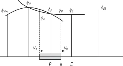
For example, when velocity through the west and east faces are greater than 0, a quadratic fit through WW (cell centroid on the upstream side), P (left bracketing cell centroid) and E (right bracketing cell centroid) is used to evaluate `ϕ _w`.

It can be shown for a uniform grid, the value of `phi` at the cell faces between two bracketing nodes i and i-1 and upstream node i-2 is given by the following formula:

`ϕ_(face)=6/8 ϕ_(i-1)+3/8 ϕ_i-1/8 ϕ_(i-2)`

This is a 3^rd order Upwind difference scheme derived as follows.

`ϕ(x)=ϕ_P+(x-x_P ) (∂ϕ)/(∂x)|_P+(x-x_P )^2/(2!) (∂^2 ϕ)/(∂x^2 )|_P+0(Δx)^3`

Discretize the first and second order derivative using Central differencing scheme and assuming F on the east face to be greater than 0.

`(∂ϕ)/(∂x)|_P=(ϕ_E-ϕ_w)/(2Δx)+0(Δx^2 )`

`(∂^2 ϕ)/(∂x^2 )|_p=(ϕ_E-2ϕ_P+ϕ_W)/(Δx^2 )+0(Δx^2 )`

`x_e=x_P+(Δx)∕2`

Substituting the discretized derivatives into the main equation, we get,

`ϕ_e=ϕ_P+((Δx)/2)((ϕ_E-ϕ_P)/(2Δx))+((Δx^2)/8)((ϕ_E-2ϕ_P+ϕ_W)/(Δx^2 ))`

Rearranging the above equation, we get,

`ϕ_e=6/8 ϕ_P+3/8 ϕ_E-1/8 ϕ_W`

CONCLUSION

QUICK scheme is conservative, in terms of TSTE it is third order accurate and conditionally bounded.

This scheme is conditionally stable.

The discretized equations involve not only immediate-neighbour nodes but also nodes upstream of neighbours. This mean Tri-diagonal matrix algorithm (TDMA) cannot be directly applied.

The QUICK differencing scheme has greater formal accuracy than the central differencing or hybrid schemes, and it retains the upwind-weighted characteristics.

The resultant false diffusion is small, and solutions achieved with coarse grids are often considerably more accurate than those of the upwind or hybrid schemes.

NEED FOR DIFFERENT INTERPOLATION SCHEMES AND FLUX LIMITERS

As we have seen from a brief discussion of few of the schemes described above, each scheme reacts in a different manner to certain properties like Conservativeness, Boundedness and Transportive Ness depending upon factors such as Peclet number, diffusion or convection dominant problems etc.

Our objective thus would be to study these behaviours for different flow and boundary conditions, and chose a scheme most appropriate.

To understand further, a more generic formula, by algebraic manipulation is written which is general enough to encompass all the schemes discussed above.

Let us assume a flow in the positive x-direction, the value of transported quantity on the east face of a one-dimensional control volume

• In standard upwind differencing (UD) scheme is

`ϕ_e=ϕ_P`

• In a linear upwind differencing (LUD) scheme is

`ϕ_e=ϕ_p+((Δx)/2) (∂ϕ)/(∂x)|_p`

Discretizing first derivative using rearward differencing scheme

`(∂ϕ)/(∂x)|_p=(ϕ_P-ϕ_W)/(Δx)`

`ϕ_e=ϕ_P+((ϕ_P-ϕ_W ))/(Δx) ((Δx)/2)`

`ϕ_e=ϕ_P+1/2 (ϕ_P-ϕ_W )`

Rearranging, it can be written as

`ϕ_e=ϕ_P+1/2 ((ϕ_P-ϕ_W)/(ϕ_E-ϕ_P ))(ϕ_E-ϕ_P )`

• In QUICK scheme is

`ϕ_e=ϕ_P+1/8 [3ϕ_E-2ϕ_P-ϕ_W ]`

Rearranging, it can be written as

`ϕ_e=ϕ_P+1/2 [(3+(ϕ_P-ϕ_W)/(ϕ_E-ϕ_P )) 1/4](ϕ_E-ϕ_P )`

• In Central Differencing (CD) scheme is

`ϕ_e=(ϕ_P+ϕ_E)/2`

`ϕ_e=ϕ_P+1/2 (ϕ_E-ϕ_P )`

Generalizing the higher-order scheme in the following form:

`ϕ_e=ϕ_P+1/2 ψ(ϕ_E-ϕ_P )`

Were `ψ` is an appropriate function.

Upon observing the above equations, we find that the ratio of upwind-side gradient to downwind-side gradient `(ϕ_P-ϕ_W )∕(ϕ_E-ϕ_P )` determines the value of function and nature of the scheme.

`r= (ϕ_P-ϕ_W )∕(ϕ_E-ϕ_P )`

For the UD scheme `ψ(r)=0`

For the CD scheme `ψ(r)=1`

For the LUD scheme `ψ(r)=r`

For the QUICK scheme `ψ(r)=(3+r)/4`

The term “TVD or total variation diminishing” dictates that the total variation of a discrete solution should diminish with time.

Necessary and sufficient conditions for a scheme to be TVD in terms or `r-Ψ` relationship:

• If 0 < r < 1 the upper limit is ψ(r) = 2r, so for TVD schemes ψ(r) ≤ 2r
• If r ≥ 1 the upper limit is ψ(r) = 2, so for TVD schemes ψ(r) ≤ 2

The idea of designing a TVD scheme is to introduce a modification to the above schemes so as to force the r–ψ relationship to remain within the shaded region for all possible values of r. This would imply that, in order to make the scheme TVD, we must constrain or limit the range of possible values of the additional convective flux which was originally introduced to make the scheme higher-order. Hence, the function ψ(r) is called a flux limiter function.

A limiter function ensures that backward- and forward-facing gradients are treated in the same fashion without the need for special coding.