Week 4 - CHT Analysis on Exhaust port

Introduction, aim and objective

Conjugate heat transfer (CHT) analysis is used were there is a temperature variation during heating or cooling of a material as a result of interaction between solid and fluid phases.

It is a transfer of heat in solids to fluids and vice versa

Some of the examples include HVAC, Heat Exchangers, Internal combustion engines, Heat sink, Boilers, Reactors, Heat pipe, Turbocharger etc.

In this challenge we shall perform a CHT analysis on the exhaust manifold model and to examine the velocity, temperature and heat transfer coefficient on the external wall.

Solving and Modelling approach

To perform CHT analysis in exhaust port simulation with ANSYS Fluent, proper setup of model geometry is imperative with good quality meshing. To compare the results and value of surface heat transfer coefficient on internal solid surface, 2 cases are performed with different solvers, namely the k-epsilon and k-omega model with proper selection of Y plus values.

Below are snippets depicting the work flow accordingly.

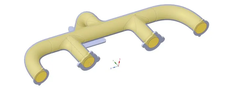
Fluid Volume

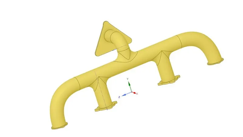
Solid Volume

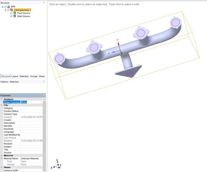
Share Topology

This is an important step as we need the a flow of information from fluid to solid region of geometry.

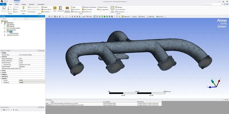
Refined Mesh

This refinement was enough to get decent answers without affecting the numerical simulation time much.

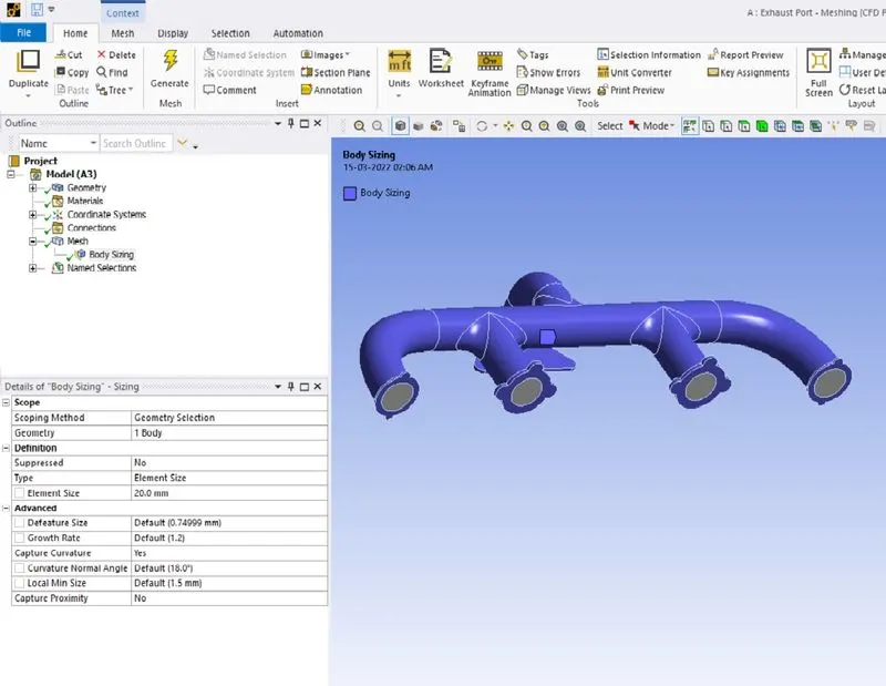
This image shows that the size of cells in solid body is refined to a better scale than cells in fluid region as we need to calculate surface heat transfer coefficient and temperature at outer walls of body.

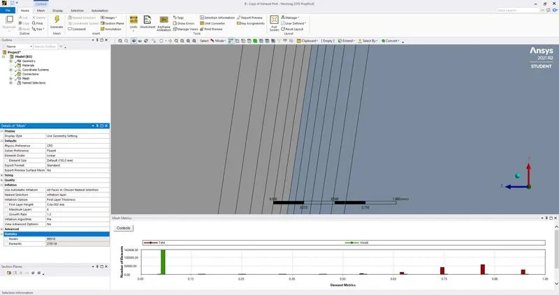
Image showing inflation layer and details

This inflation layer is used only for k-omega SST solver, this image shows the first layer thickness which is taken from a Y plus value of 1. A snippet for the same is shown in ensuing paras. The calculation of first layer thickness is done using a standard site.

Pre-processing and solver setting

Here we shall be setting up the physics of the problem for simulation.

Enable energy equation under physics tab, in Models ribbon.

Next, open viscous option under Models and see to it that k-epsilon model is selected.

Under Zones ribbon, open cell zones and see to it that fluid zone is set to fluid and solid zone is selected as solid.

Under materials ribbon, verify that the solid we will be using is Aluminium (this will be selected as a default).

Under zones ribbon, open boundaries, here we shall be having a number of boundaries. These are discussed below.

• Inlet – These as the name suggest, are the inlet boundaries of the exhaust gases.
• Interior-final geometry_1-fluid_volume - These comprise of cells in fluid region.
• Interior-final geometry_1-solid_volume: These comprise of cells in solid region.
• Outer-wall-convection: This is the outer wall.
• Wall-final-geometry_1-fluid-volume-final_geometry_1-solid_volume:

This is the internal wall, which is an interface at the fluid side.

• Wall-final-geometry_1-fluid-volume-final_geometry_1-solid_volume-shadow:

This is the internal wall, which is an interface at the solid side.

• What is a shadow boundary wall?

When you read a mesh with a 2-sided wall zone (which forms the interface between solid/fluid regions) into ANSYS FLUENT, a ‘shadow’ zone will automatically be created so that each side of the wall is a distinct wall.

The face of the solid domain will be ‘shadow wall’, and the face of the fluid domain will be ‘wall’.

• Wall-final_geometry_1-solid-volume:

These are the flanges at the inlet and outlet. These are considered to be adiabatic in nature (no transfer of heat).

Inlet Boundary Condition taking a velocity inlet value of 5 meter per second

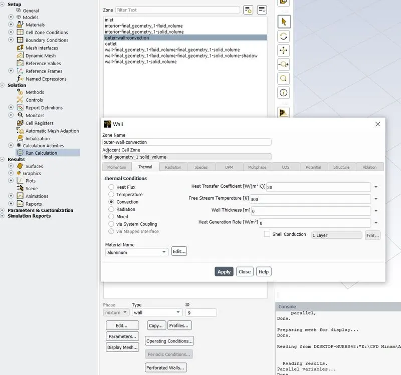
outer-wall-convection having heat transfer coefficient value of 20

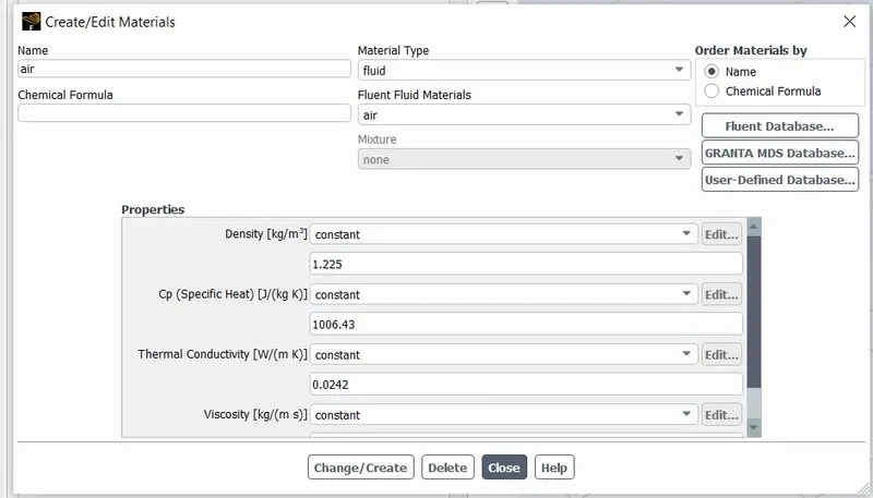
properties of fluid - these are used to calculate Reynolds, Prandtl and Nusselt number

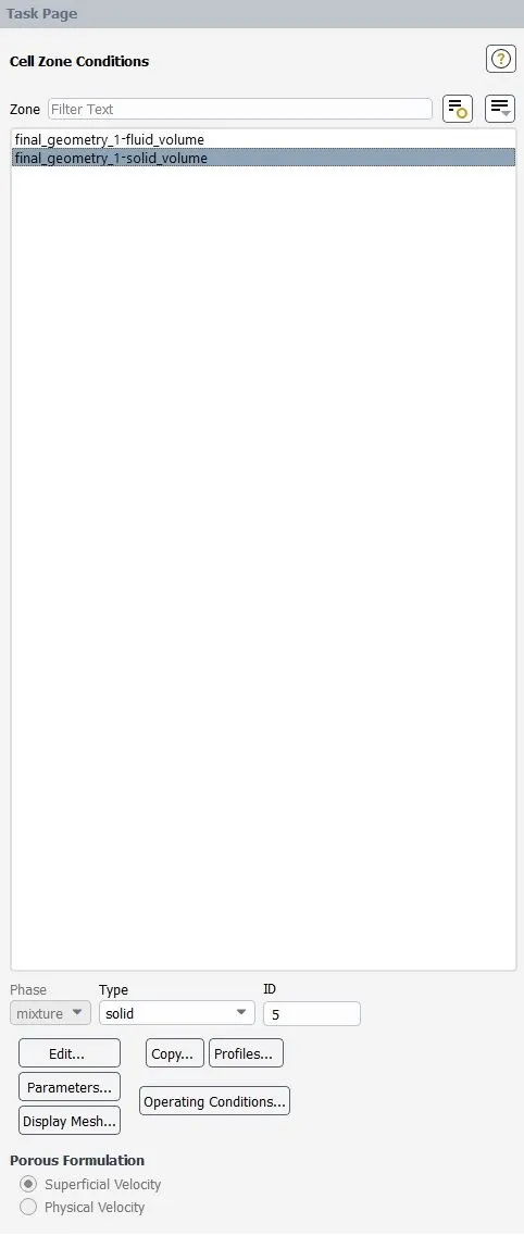
solid zone cells

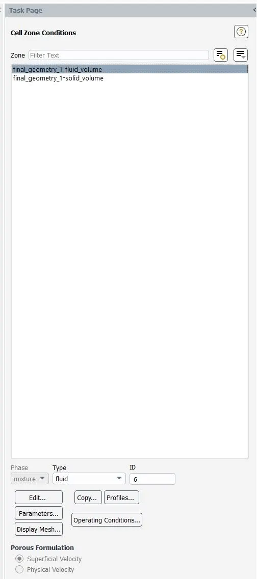
fluid zone cells

These 2 images are included as it is imperative to define the solid wall as solid and inner zone as fluid, missing out on this leads to errors.

htc contour

Image to show creation of heat transfer coefficient contour

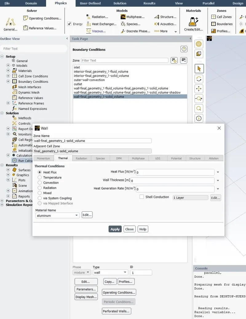
adiabatic flanges

Image showing how to model an adiabatic wall

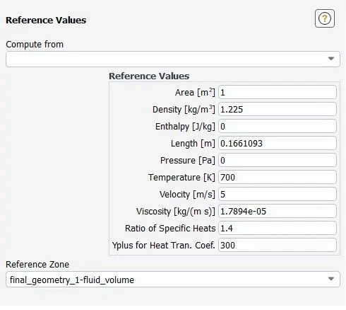
Reference values

These values are important to cacluate the correct values of heat transfer coefficient

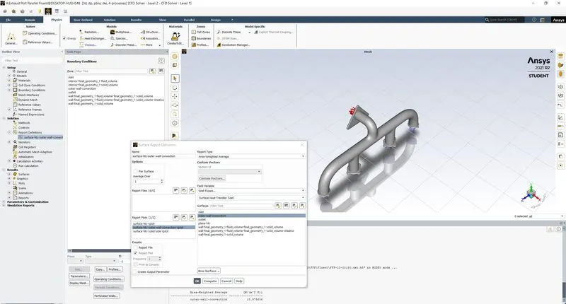
Surface heat transfer coefficient definition report

Image showing how to model a plot for heat transfer coefficient.

Analytical method to calculate heat transfer coefficient:

In order to calculate the heat transfer coefficient, the Dittus Bolter heat transfer coefficient relation is used to determine the Nusselt number which is given mathematically as

`Nu_D=0.023*Re_d^(4/5)*Pr^n`

Were Re is Reynolds number

Pr is Prandtl number.

Reynold number is the ration of inertial to viscous forces. This dimensionless number determines which forces are more prevalent at a particular location, a higher Reynolds number tells us that the inertial forces are more dominant in the fluid flow region.

Likewise, Prandtl number is also a dimensionless number, which is a ratio of the hydrodynamic boundary layer to the viscous boundary layer.

Calculation of Prandtl number:

A higher value of Prandtl number tells us that viscous layer is more dominant than the heat transfer capacity of the same fluid. This can also be given as a ratio of kinematic viscosity to thermal diffusivity. Upon substituting their values, we get the equation for Prandtl number as below

`Pr⁡=(μ*C_p)/k_f`

Were, `mu` = dynamic viscosity of the fluid in kg per meter second = 1.7894s-05

`K_f` = thermal conductivity of the fluid (air in our case) = 0.0242 Watts per meter kelvin

`C_p` = Specific heat of fluid = 1006.43 joules per kg kelvin

Prandtl number comes to about 0.744176

Calculation of Reynolds number:

`Re=(ρ*V*D_h)/μ`

Were,

`D_h` = hydraulic Diameter = 4*cross sectional area / perimeter

And `\rho` is the density.

Diameter of the inlet pipe can be ascertained from the geometry in SpaceClaim.

A snippet for the same is shown below.

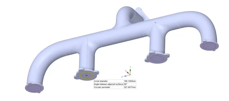
Inlet Diameter

Diameter of inlet pipe is 166.1093 mm; diameter of outlet port is 150 mm. we shall consider the greater value of the two as this gives us a higher value of Reynolds number.

Reynolds number comes to about 56858.1347.

The same can be calculated while ascertaining the delta y values against Y plus numbers.

A snippet for the same is shown below.

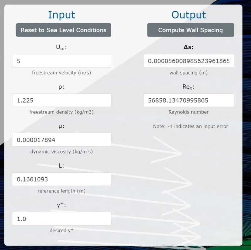
first layer thickness for yplus of one

Once Nusselt number is calculated, we can use the basic equation for Nusselt number as

`Nu=(h*L)/k`

To calculate heat transfer coefficient, h.

L is hydraulic diameter, is the diameter of inlet pipe, 166.1093 mm.

This gives us a value of h = 19.5202

Results:

CASE 1 : K-Epsilon

the snippets from the results of the simulation are attached below,

First off, we have taken the baseline model employing k-epsilon model without any inflation layers. The results having velocity, temperature contours, surface heat transfer coefficient plots are attached herein, these can be cross verified with the analytical results.

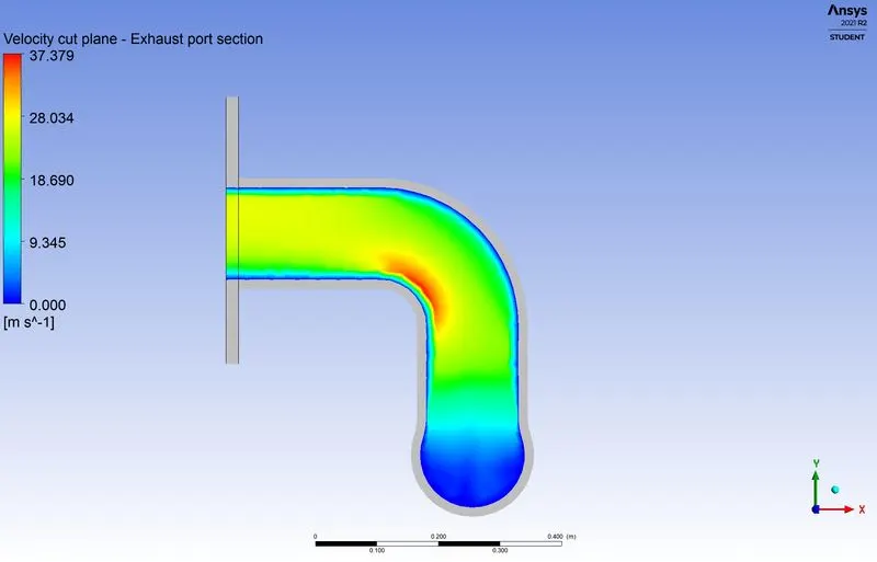
Velocity cut plane z

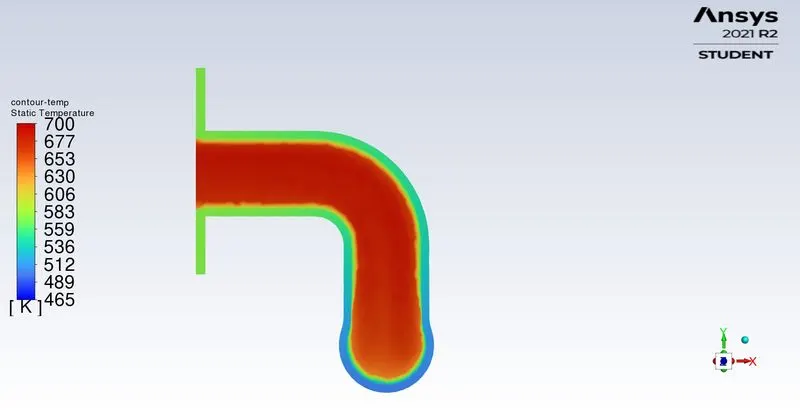
Temperature cut plane z

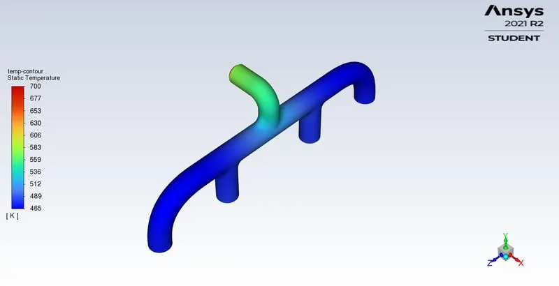
Temperature contour

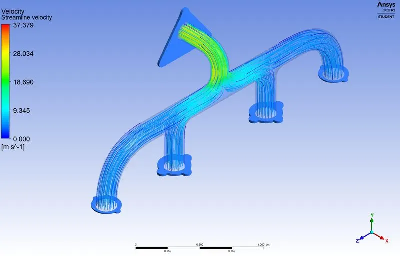
Velocity streamline

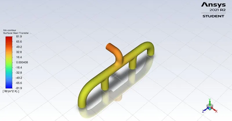
surface htc contour

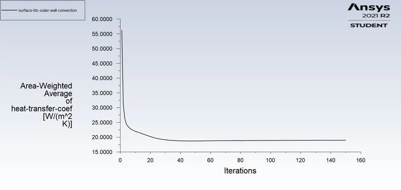
surface htc plot

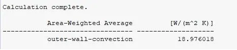
surface htc value

CASE 2 : K-Omega SST

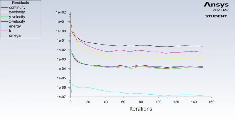
Residuals

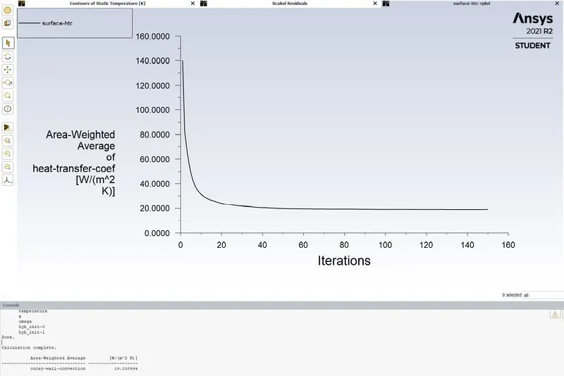
surface htc value = 19.038994

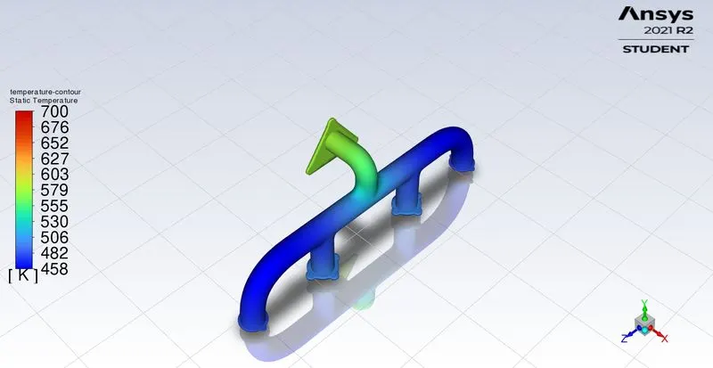
Temperature contour

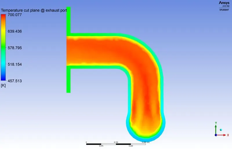
Temperature cut plane outlet

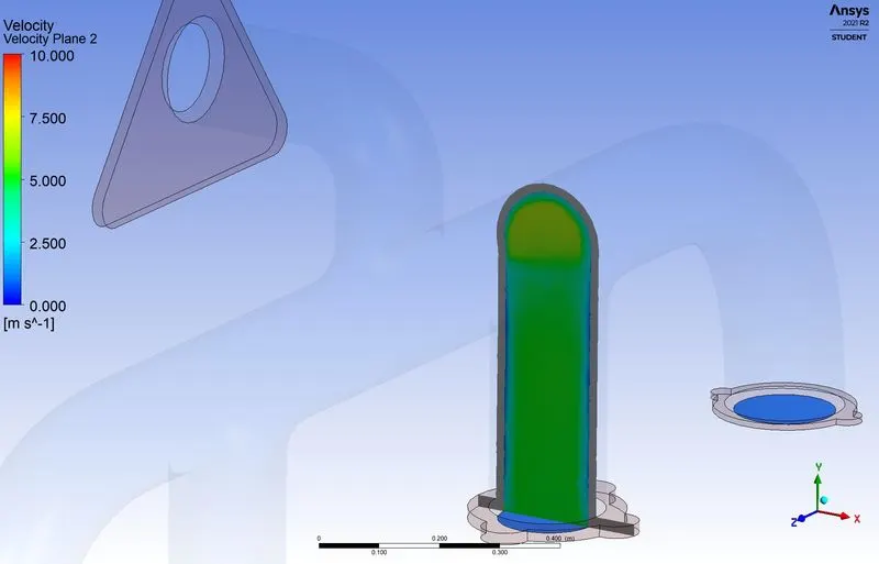
Velocity cut plane inlet

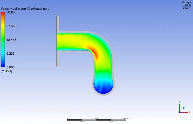
Velocity cut plane outlet

Conclusion:

CHT analysis was successfully conducted in Fluent. A pressure based, coupled scheme solver was used. Two solvers were used, k-epsilon and k-omega SST as per Y plus values.

Analytical value of heat transfer coefficient is 19.5202.

The deviation from analytical results was found to be within 5 percent, thus validating our simulation results.

Value of heat transfer coefficient is located in cell adjacent to wall, this allows us to choose a value of Y plus equal to 1 as this is in viscous sub layer, and solver as k-omega SST accordingly.

Accuracy of heat transfer coefficient depends on selecting a suitable value of Y plus as well as solver.