Week 12 - Validation studies of Symmetry BC vs Wedge BC in OpenFOAM vs Analytical H.P equation
Week 12 - Validation studies of Symmetry BC vs Wedge BC in OpenFOAM vs Analytical H.P equation
In this project, we shall not be performing analysis on the complete circular cross section of a pipe, rather we shall be considering different sizes of the section of circular cross section of pipe for analysis and simulation.
Comparisons and inferences from observations between various sizes applying different boundary conditions shall be documented accordingly.
We shall be considering 3 different angles (10 degrees, 25 degrees and 45 degrees) and applying both wedge and well as symmetry boundary conditions to the cut walls. Differences between the two types of boundary conditions shall be noted down.
Before we start with choosing the dimensions of the geometry and various physics of the problem, we need to understand wedge and symmetry boundary conditions.
Wedge Boundary condition:
The wedge boundary condition (BC) is used in computational fluid dynamics to define an axisymmetric situation, for e.g., cylinder. The model and flow must be axisymmetric along a central line such that all physical variables of the flow have the same value and distribution at a given radius for all angles.
This boundary condition is specified by two planes that must be selected on separate sides of the domain (referred to as front and back) on surfaces running along the axis. It works for 2D simulations only.
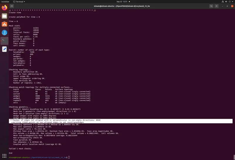
As an example, focus on the snippet of OpenFOAM checkmesh result below, when a wedge boundary condition is employed, the angles are divided equally from the centre line, onto both sides of the domain.
The below example is for a wedge angle of 45 degrees, two planes on either side of the domain are divided equally into 22.5 degrees each.
An important point to be noted:
If number of cells are increased to a value of more than one in z-direction while using wedge boundary conditions, then even if the application (icoFoam) runs, we still are faced with an error in checkMesh command in terminal. A snippet of the same is shown below.
Wedge is different from the symmetry boundary condition in the sense that the wedge BC applies the Navier-Stokes equations in cylindrical coordinates whereas the latter applies N-S equations in cartesian coordinates.
One big advantage of wedge is that it allows for the rotational flow around the axis and this is possible only because the fluxes and normal components are not assumed as zero.
Symmetry Boundary condition:
The symmetry boundary condition defines a mirror face/surface. It should only be used if the physical object or geometry and the expected flow field pattern of the developed solution are mirrored along that surface. By using this boundary condition, the domain can essentially be halved, reducing the time to achieve a solution.
In detail, the symmetry condition applies the following constraints on the flow variables:
- The fluxes across the symmetry are zero.
- The normal components of all variables are set to zero.
It can be applied to both planar or non-planar faces/surfaces on the domain boundaries.
Basic boundary conditions in CFD
When we are doing CFD, we are doing a flow simulation on object that represents the fluid. There are 3 very basic boundary conditions in CFD, first being velocity inlet, how flow moves into flow domain.
Second one is pressure outlet. How and where flow moves out of the pipe. Third is wall condition, where there is a physical condition in the flow where fluid cannot pass and flow only in a direction parallel to it.
Physics of the flow
Pipe Diameter = 2 cm
Pipe Length = 3 meters
Fluid = Water
Reynolds number = 2100
Entrance length = 2.1 meters
Formulas:
Entrance length:
`L=0.05*D*Re`
Reynold Number:
`Re=(ρ*U*D)/μ`
Velocity distribution in FDF Region
`V_r=R^2/((4μU_(avg) ) )*((dp)/dz)*(1-(r^2/R^2 ))`
When r = 0; we have our maximum velocity, thus our equation becomes:
`V_r=V_max*(1-(r^2/R^2 ))`
Pressure-drop:
`∆P=(32.μ.U_(avg).L)/D`
Kinematic viscosity:
`ν=μ/ρ`
Flow is laminar.
Understanding MATLAB file:
In this script, I have started with all the basic inputs required to solve the HP equations. Kinematic viscosity, Pressure drop and maximum velocity are calculated.
Average velocity is calculated using Reynolds number equation.
Data was extracted from OpenFOAM and read into the script. This included data for velocity variation in radial direction in the fully developed flow region, maximum velocity variation along the axis in FDF Region, pressure variation across the length of fully developed flow region and Shear Stress variation at a distance of 2.1 meter which falls under the fully developed flow region.
Observations and Inferences from velocity distribution at 2.1 meters (Fully Developed Flow region)
- An angle of 10 and 25 theta when symmetry boundary condition is applied, are the closest to the analytical plot, near the walls of the pipe.
- Though as the angle increases to 45 degrees, we see the variation is greater but acceptable when compared to wedge condition for the same angle.
- When comparing the wedge boundary conditions, it has been observed that 10 degrees is closer to the analytical plot than 25 and 45 degrees.
- The most to digress from the analytical plot is 25- and 45-degrees theta when wedge boundary condition is used, 45 degrees wedge being the farthest.
- In Conclusion, 10- and 25-degrees symmetry boundary condition gave the closest answers with 45 degrees wedge being the worst-case scenario.
- Thus, wedge case, as mentioned in paras above, is best when used in angles less than 5 degrees. As the angles are increased in magnitude, the numerical values digress away from analytical values in greater values.
- The number of cells in z-direction, in case of symmetry boundary conditions are also a deciding factor. Greater the number of cells, smoother will be the result. But it should also be noted that the courant number should be kept in check. Also, the simulation time increases by increasing the number of cells in z-direction.
- Overall, symmetry boundary condition, with 25 degrees wedge angles gave the best solution, this being the closest to the analytical plot.
- The zoomed plot below gives in a better insight on the matter.
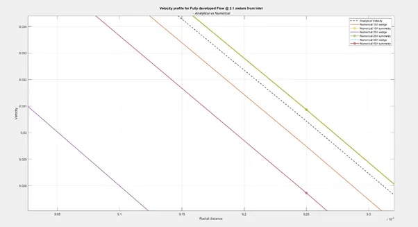
MATLAB script file for the plot and all supporting documents will be attached at the end of report.
Observations and Inferences from shears stress distribution at 2.1 meters (Fully Developed Flow region)
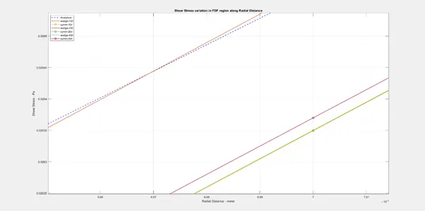
- For a 10 mm radius pipe, Wedge boundary condition at 10 degrees wedge angle is closer to analytical value up to 7 mm.
- A wedge boundary condition with wedge angle of 25 degrees gives fairly accuarate answers up till a radial distance of 4 mm, following which, it diverts further away.
- All the three angles of 10,25 and 45 degrees used in symmetry boundary condition give us values closest to analytical profile.
- Wedge boundary condition with wedge angle of 45 degrees proves to be the worst-case scenario, similar to the velocity distribution in FDF Region case.
- In conclusion, a 10 degrees wedge angle with wedge boundary condition gives fairly closer results, thus, wedge boundary condition can be used but, as stated, it should have an angle of less than 5 degrees.
- A zoomed image is shown below:
References:
- https://www.simscale.com/docs/simulation-setup/boundary-conditions/symmetry/
- https://www.simscale.com/docs/validation-cases/compressible-flow-de-laval-nozzle/
- https://www.simscale.com/docs/simulation-setup/boundary-conditions/
- https://www.cfdsupport.com/OpenFOAM-Training-by-CFD-Support/node94.html
- https://skill-lync.com/student-projects/Pipe-flow-simulation-in-OpenFOAM-Part-22-Symmetry-boundary-conditions-72117
- https://skill-lync.com/knowledgebase/how-to-mirror-results-in-paraview
Details of 10 theta wedge angle using wedge boundary conditions
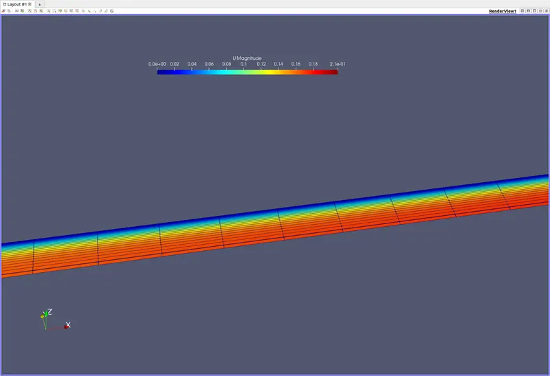
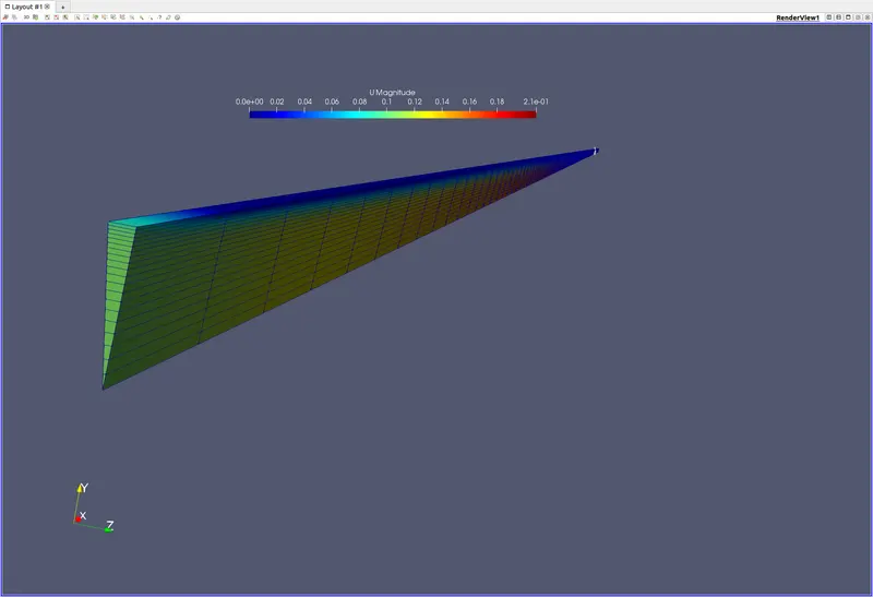
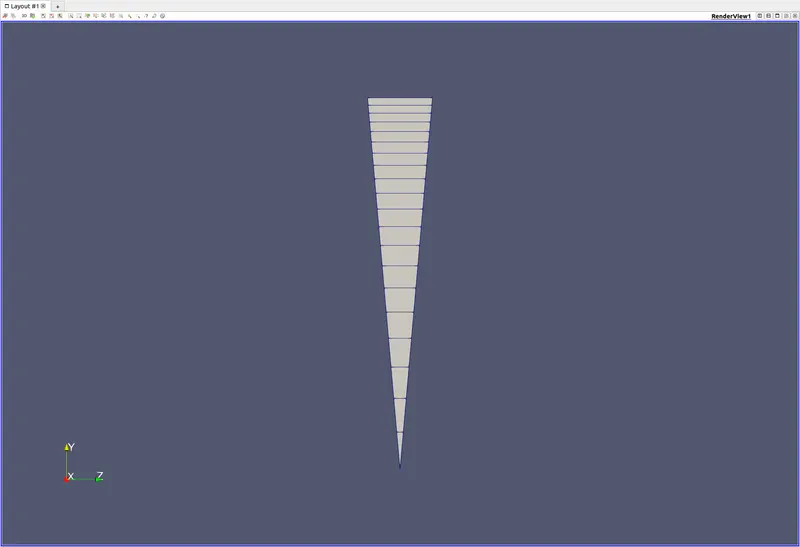
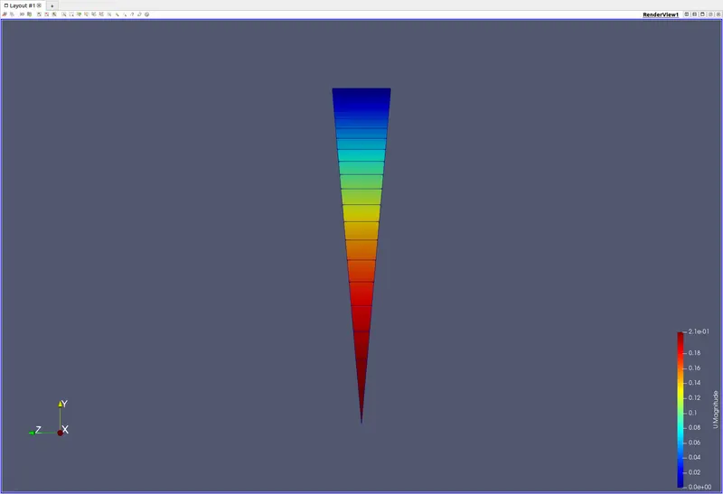
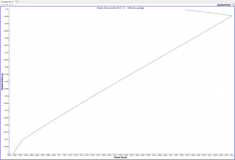
- Shear Stress variation @ 2.1 meters from Inlet
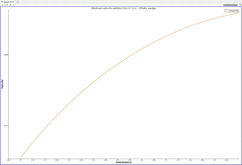
- U_max variation in FDF Region
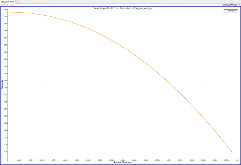
- U variation @ 2.1 meters
Details of 10 theta wedge angle using symmetry boundary conditions
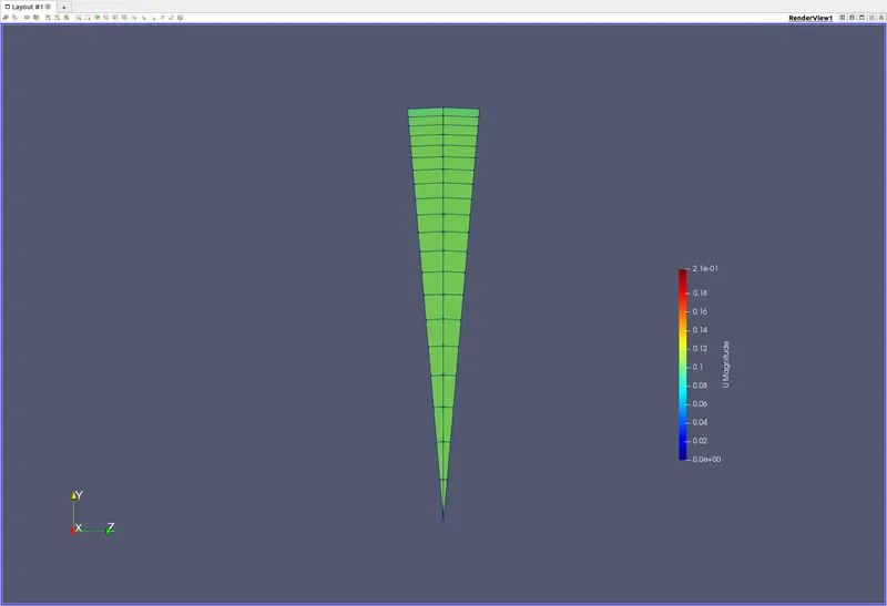
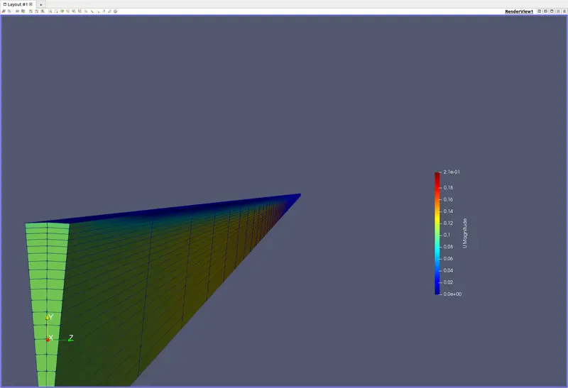
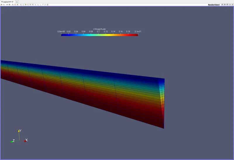
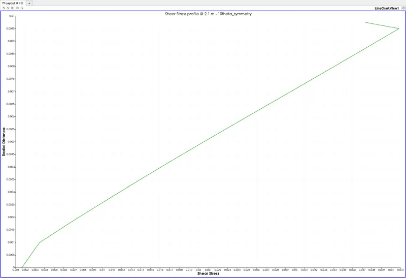
- Shear Stress variation @ 2.1 meters from Inlet
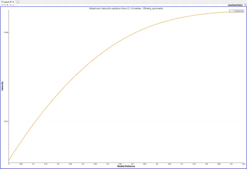
- U_max variation in FDF Region
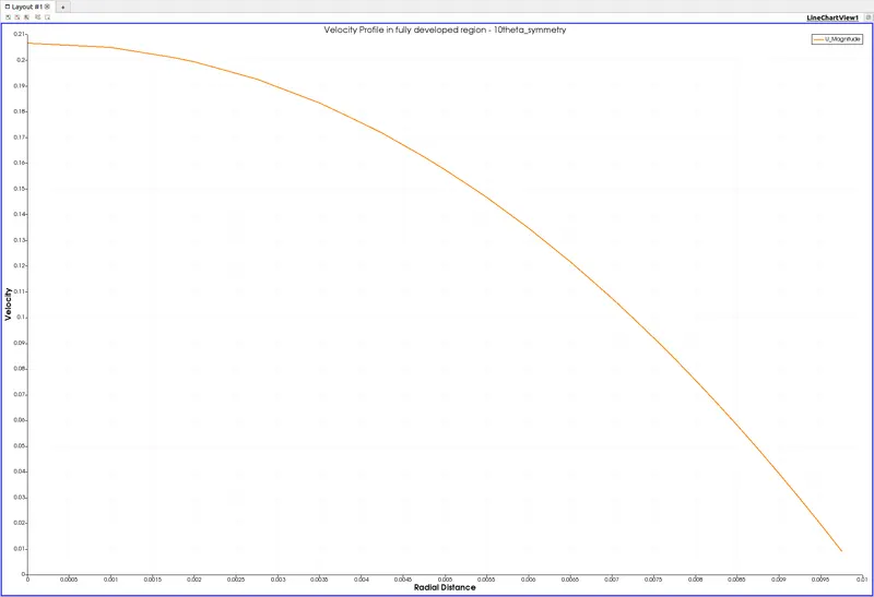
- U variation @ 2.1 meters
Details of 25 theta wedge angle using wedge boundary conditions
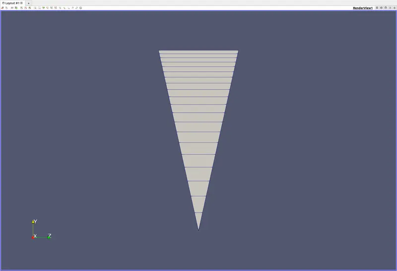
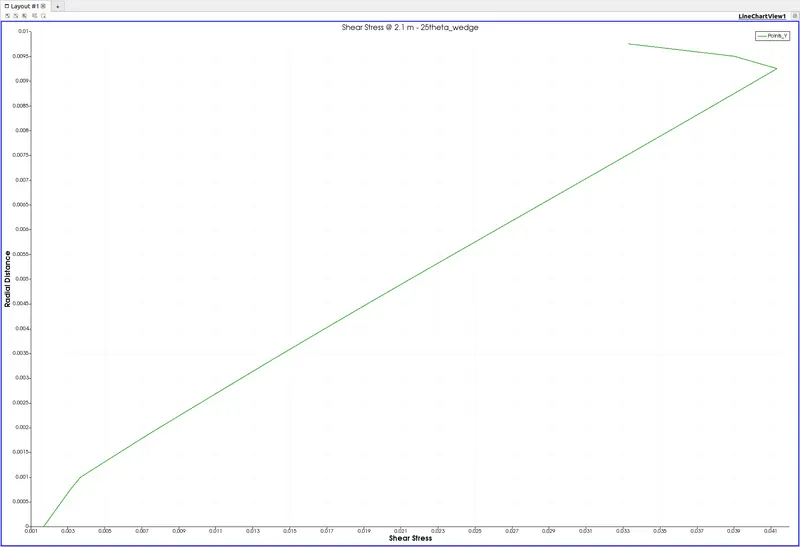
- Shear Stress variation @ 2.1 meters from Inlet
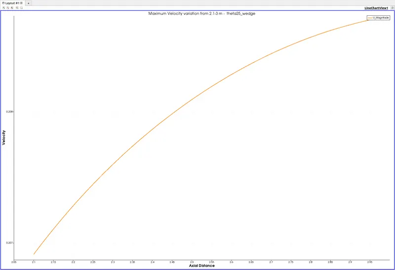
- U_max variation in FDF Region
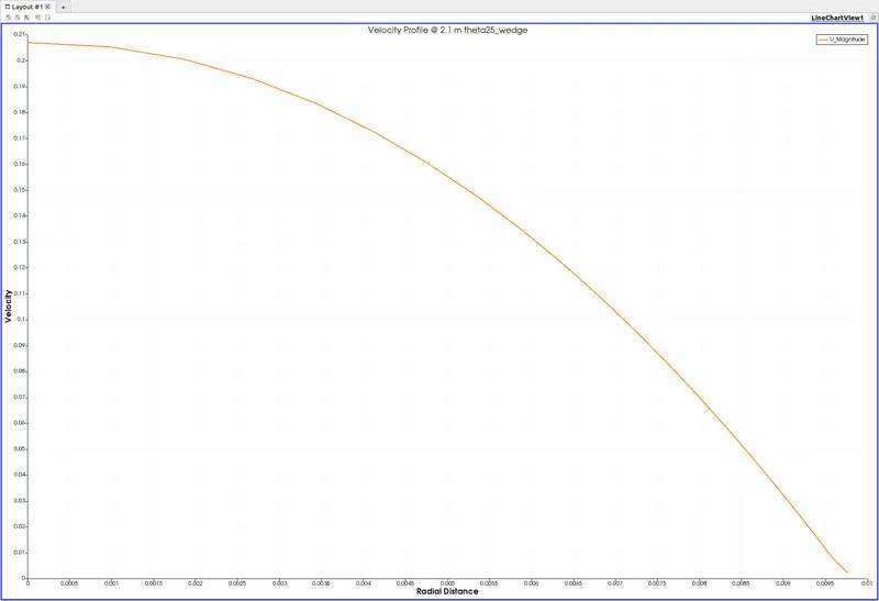
- U variation @ 2.1 meters
Details of 25 theta wedge angle using symmetry boundary conditions
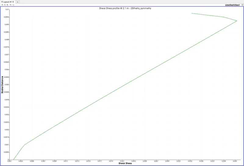
- Shear Stress variation @ 2.1 meters from Inlet
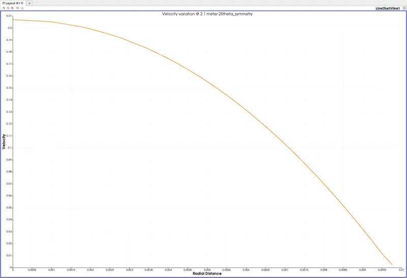
- U variation @ 2.1 meters
Details of 45 theta wedge angle using wedge boundary conditions
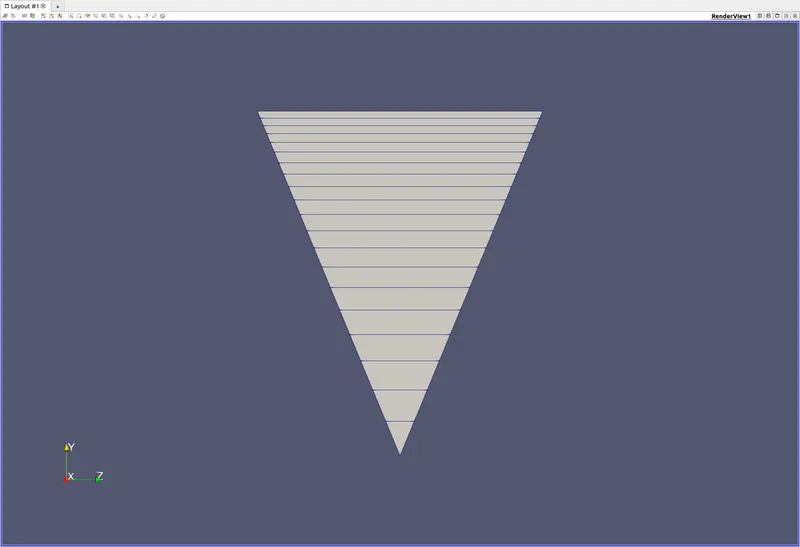
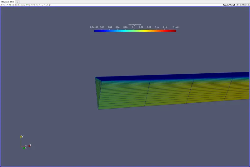
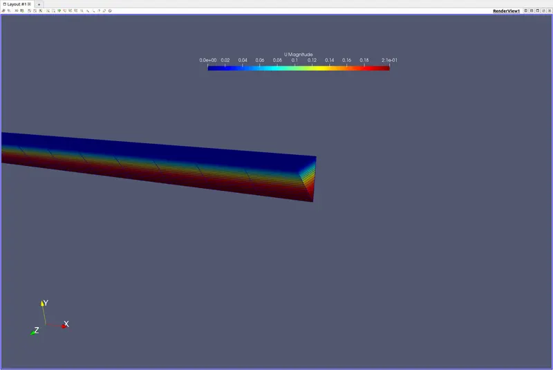
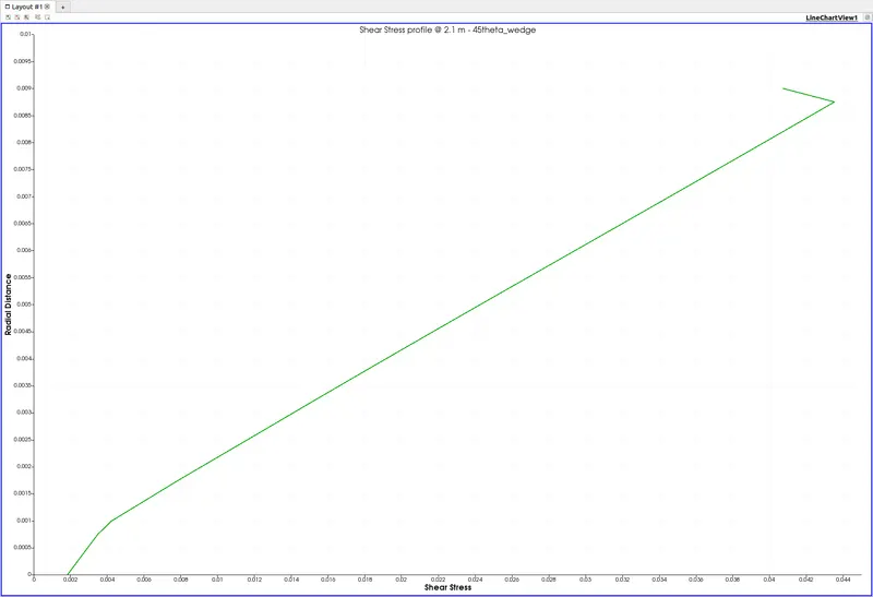
- Shear Stress variation @ 2.1 meters from Inlet
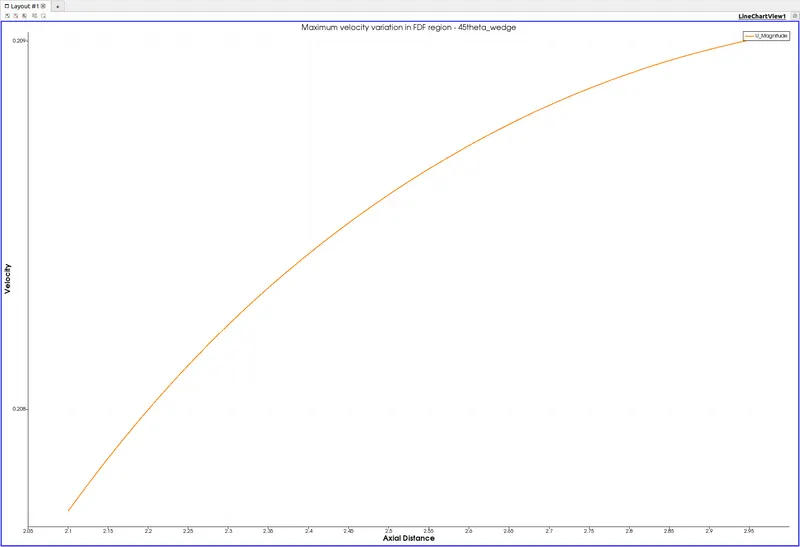
- U_max variation in FDF Region
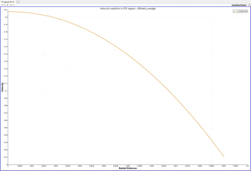
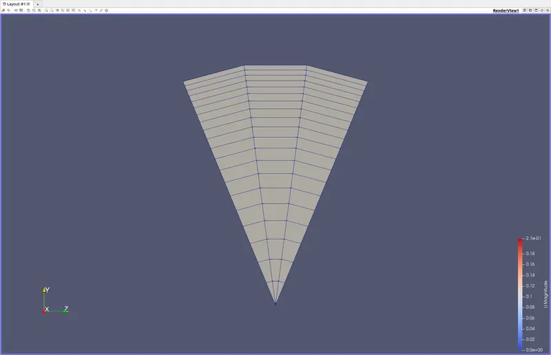
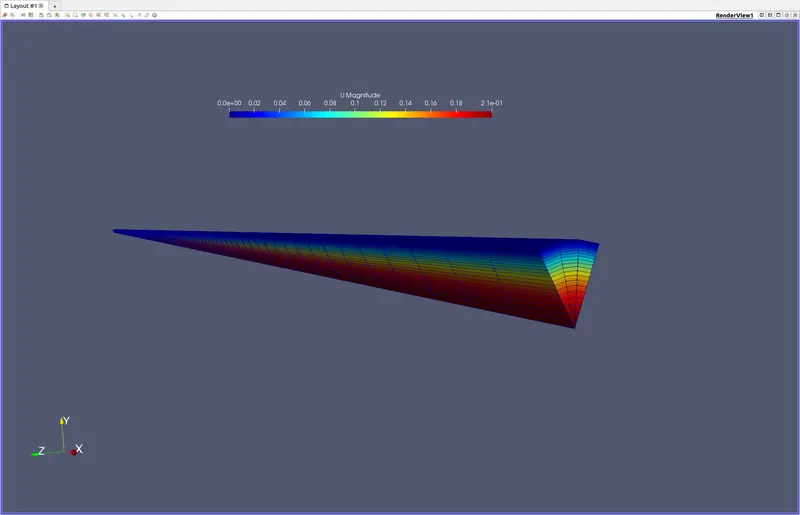
Details of 45 theta wedge angle using symmetry boundary conditions
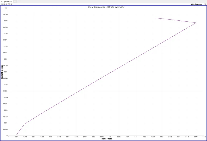
- Shear Stress variation @ 2.1 meters from Inlet
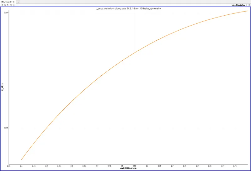
- U_max variation in FDF Region
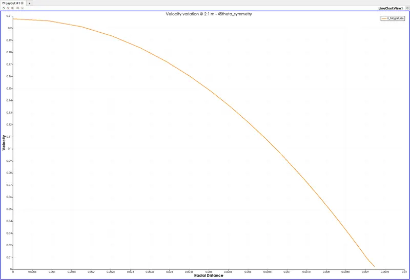
- U variation @ 2.1 meters
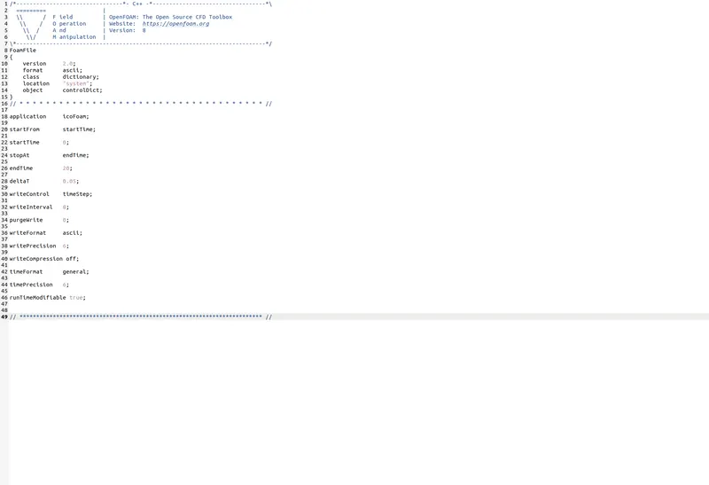
- controlDict file
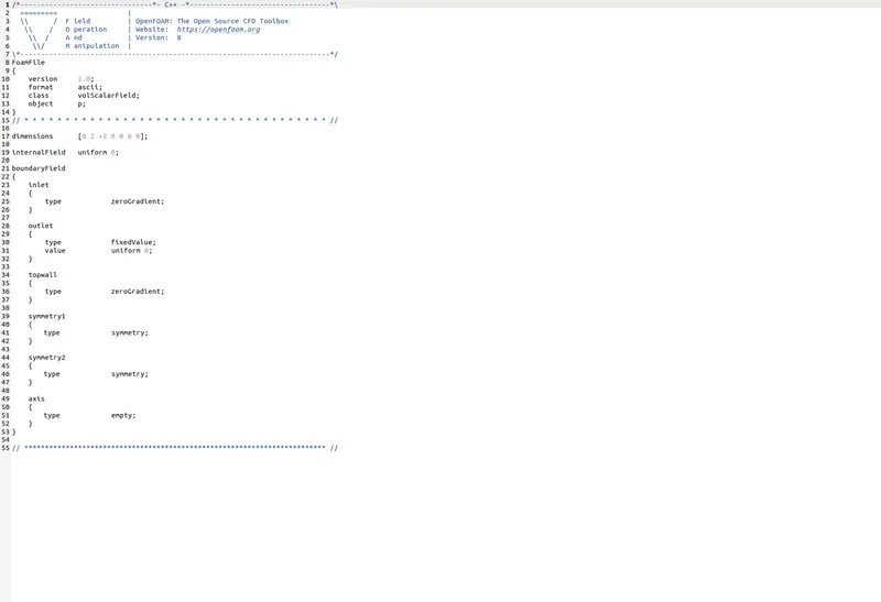
- p file
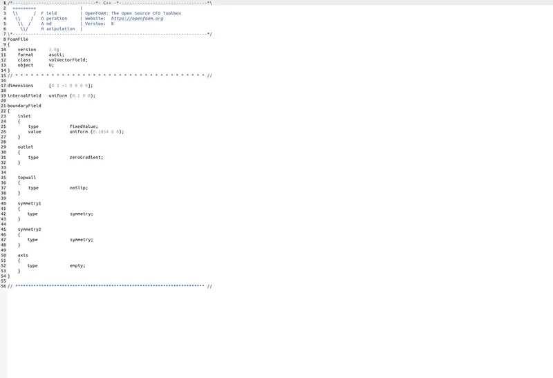
- U file
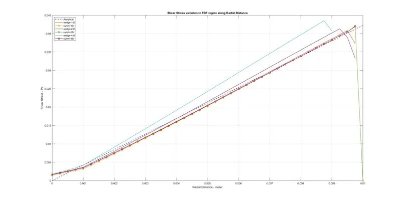
- Shear Stress variation in Fully Developed Flow Region
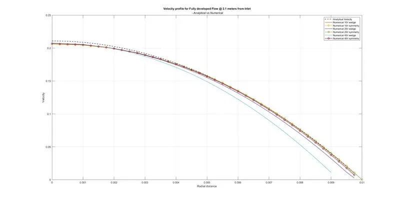
- U_velocity variation @ 2.1 meters from Inlet
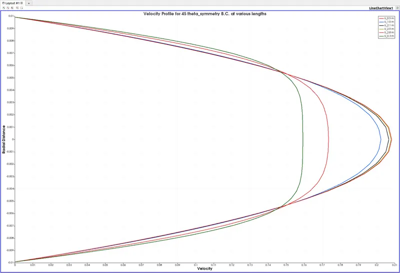
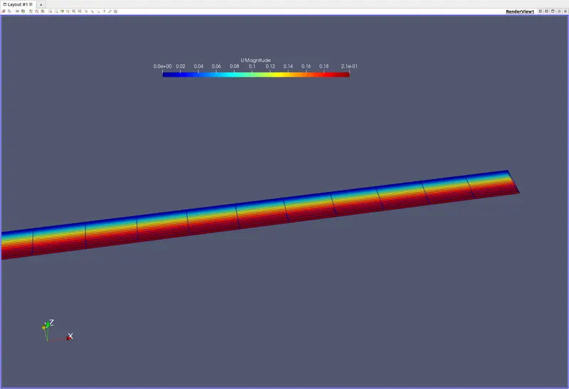
- Velocity Profiles at various distances along length of the pipe for a 45 degree wedge angle and symmetry boundary condition.
- MATLAB script to calculate analytical values with plots and tables for comparisions
clear all
close all
clc

%% Inputs

Re = 2100; % Reynolds number-Dimensionless
rho = 998.21; % Density-m3/s
mu = 1.002e-3; % Dynamic viscosity-N-s/m2
D = 0.02; % Diameter
R = D/2; % Radius
L_e = 0.05*D*Re; % Hydrodynamic entrance length
L = round(L_e+1); % Total length of the pipe
L_FD = L-L_e; % Length of fully developed flow region
nu = mu/rho; % kinematic viscosity

% Average velocity in pipe for a fully developed flow
% Re = rho*V*D/mu
V = (Re*mu) / (rho*D); % m/s
% Maximum velocity in the pipe
V_max_analytical = 2*V; % m/s
% Pressure drop from Hagen Poiseuille's equation
delta_P = 32*mu*L_FD*V/(D^2); % Pa
% Kinetic Pressure drop
delta_P_K = delta_P/rho; % (m/s)^2

%% Extracting Data from Excel files

% Extracting velocity and shear stress profile @ 2.1 m from excel

U_tau_4_wedge = xlsread('U @ 2.1 m  from inlet_4theta_wedge.csv');

U_tau_10_wedge = xlsread('U_&_tau @ 2.1m_10theta_wedge.csv');
U_tau_10_symmetry = xlsread('U_&_tau @ 2.1m_10theta_symmetry.csv');

U_tau_25_wedge = xlsread('U_&_tau @ 2.1m_25theta_wedge.csv');
U_tau_25_symmetry = xlsread('U_&_tau @ 2.1m_25theta_symmetry.csv');

U_tau_45_wedge = xlsread('U_&_tau @ 2.1m_45theta_wedge.csv');
U_tau_45_symmetry = xlsread('U_&_tau @ 2.1m_45theta_symmetry.csv');

% Extracting U_max and pressure data 2.1-3 meter from excel

data_U_max_10_wedge = xlsread('U_max 2.1-3 m 10theta_wedge.csv');
data_U_max_10_symmetry = xlsread('U_max & pressure drop in FDF Region 10theta_symmetry.csv');

data_U_max_25_wedge = xlsread('U_max 2.1-3 m 25theta_wedge.csv');
data_U_max_25_symmetry = xlsread('U_max 2.1-3 m 25theta_symmetry.csv');

data_U_max_45_wedge = xlsread('U_max 2.1-3 m 45theta_wedge.csv');
data_U_max_45_symmetry = xlsread('U_max and pressure drop @ 2.1-3 m 45theta_symmetry.csv');

%% 1 - Validate Maximum velocity with HP Equations

% Check for variation of maximum velocity in FDF Region with analytical velocity

U_max_10_wedge = data_U_max_10_wedge(:,2);
U_max_10_symmetry = data_U_max_10_symmetry(:,2);
U_max_25_wedge = data_U_max_25_wedge(:,2);
U_max_25_symmetry = data_U_max_25_symmetry(:,2);
U_max_45_wedge = data_U_max_45_wedge(:,2);
U_max_45_symmetry = data_U_max_45_symmetry(:,2);

U_max_10_wedge_average = mean(U_max_10_wedge);     % 10 degrees theta
U_max_10_symmetry_average = mean(U_max_10_symmetry);
U_max_25_wedge_average = mean(U_max_25_wedge);     % 25 degrees theta
U_max_25_symmetry_average = mean(U_max_25_symmetry);
U_max_45_wedge_average = mean(U_max_45_wedge);     % 45 degrees theta
U_max_45_symmetry_average = mean(U_max_45_symmetry);

% Table to check variation of maximum velocity in fully developed flow
% region in axial direction

Type = {'Analytical-HP Equations';'Num_theta10_wedge';'Num_theta10_symmetry';...
    'Num_theta25_wedge';'Num_theta25_symmetry';'Num_theta45_wedge';'Num_theta45_symmetry'};
U_max = [V_max_analytical;U_max_10_wedge_average;U_max_10_symmetry_average;...
    U_max_25_wedge_average;U_max_25_symmetry_average;U_max_45_wedge_average;...
    U_max_45_symmetry_average];

error_10_wedge = ((V_max_analytical-U_max_10_wedge_average)/V_max_analytical)*100;
error_10_symmetry = ((V_max_analytical-U_max_10_symmetry_average)/V_max_analytical)*100;

error_25_wedge = ((V_max_analytical-U_max_25_wedge_average)/V_max_analytical)*100;
error_25_symmetry = ((V_max_analytical-U_max_25_symmetry_average)/V_max_analytical)*100;

error_45_wedge = ((V_max_analytical-U_max_45_wedge_average)/V_max_analytical)*100;
error_45_symmetry = ((V_max_analytical-U_max_45_symmetry_average)/V_max_analytical)*100;

Variation_percentage = [NaN;error_10_wedge;error_10_symmetry;error_25_wedge;error_25_symmetry;...
    error_45_wedge;error_45_symmetry];

T1 = table(Type,U_max,Variation_percentage);
T1.Properties.Description = ['Table for Variation of maximum velocity in FDF '...
    'region for different boundary types'];
display(T1.Properties.Description)
display(T1)

%% 2 - Validate the fully developed flow velocity profile with its analytical profile

% Velocity profile @ 2.1 meter using analytical formula
r = linspace(0,R,41);
[V_r] = V_max_analytical*(1-(r.^2./R^2)); % Analytical values

U_4_wedge = U_tau_4_wedge(:,1);

U_10_wedge = U_tau_10_wedge(:,1);
U_10_symmetry = U_tau_10_symmetry(:,1);

U_25_wedge = U_tau_25_wedge(:,1);
U_25_symmetry = U_tau_25_symmetry(:,1);

U_45_wedge = U_tau_45_wedge(:,1);
U_45_symmetry = U_tau_45_symmetry(:,1);

% Table 2 - Table documenting velocity profile values @ 2.1 meter

T2 = table(r',V_r',U_10_wedge,U_10_symmetry,U_25_wedge,U_25_symmetry,U_45_wedge,U_45_symmetry);
T2.Properties.VariableNames = {'Radius','U_analytical','U_10theta_wedge','U_10theta_symmetry',...
    'U_25theta_wedge','U_25theta_symmetry','U_45theta_wedge','U_45theta_symmetry'};
T2.Properties.Description = 'Table documenting velocity profile values @ 2.1 meter';
display(T2.Properties.Description)
display(T2)

% Creating plot to compare velocity profile @ FDF

figure('name','Velocity profile in FDF Region - Analytical vs Numerical','windowstate','maximized')
plot(r,V_r,'k--',r,U_4_wedge,'-*',r,U_10_wedge,r,U_10_symmetry,'-o','linewidth',1.2)
hold on
plot(r,U_25_wedge,r,U_25_symmetry,'-o',r,U_45_wedge,r,U_45_symmetry,'-o','linewidth',1.2)
xlabel('Radial distance')
ylabel('Velocity')
[t,s] = title('Velocity profile for Fully developed Flow @ 2.1 meters from Inlet',...
    ' - Analytical vs Numerical');
s.FontAngle = 'italic';
grid on
legend('Analytical Velocity','Numerical 4\theta wedge','Numerical 10\theta wedge','Numerical 10\theta symmetry',...
    'Numerical 25\theta wedge','Numerical 25\theta symmetry','Numerical 45\theta wedge',...
    'Numerical 45\theta symmetry')
hold off

%% 3 - Validate pressure drop for fully developed flow

% Table documenting pressure drop for various types of boundary conditions

Name = {'Analytical';'10theta_wedge';'10theta_symmetry';'25theta_wedge';'25theta_symmetry';...
    '45theta_wedge';'45theta_symmetry'};
delta_P1 = [delta_P_K;data_U_max_10_wedge(1,2);data_U_max_10_symmetry(1,2);data_U_max_25_wedge(1,2);data_U_max_25_symmetry(1,2);...
    data_U_max_45_wedge(1,2);data_U_max_45_symmetry(1,2)];

P_error_10_wedge = ((data_U_max_10_wedge(1)-delta_P_K)/delta_P_K)*100;
P_error_10_symmetry = ((data_U_max_10_symmetry(1)-delta_P_K)/delta_P_K)*100;

P_error_25_wedge = ((data_U_max_25_wedge(1)-delta_P_K)/delta_P_K)*100;
P_error_25_symmetry = ((data_U_max_25_symmetry(1)-delta_P_K)/delta_P_K)*100;

P_error_45_wedge = ((data_U_max_45_wedge(1)-delta_P_K)/delta_P_K)*100;
P_error_45_symmetry = ((data_U_max_45_symmetry(1)-delta_P_K)/delta_P_K)*100;

error_pressuredrop = [NaN;P_error_10_wedge;P_error_10_symmetry;P_error_25_wedge;...
    P_error_25_symmetry;P_error_45_wedge;P_error_45_symmetry];

T3 = table(Name,delta_P1,error_pressuredrop);
T3.Properties.VariableNames = {'Type','Pressure Drop','Percentage Variation'};
T3.Properties.Description = 'Table documenting pressure drop for different boundary conditions in FDF Region';
display(T3.Properties.Description)
display(T3)

%% 4 - Validate wall shear stress for fully developed flow

% Fully developed flow starts from 2.1 m till 3 meter
% Divide it into 41 parts
% tau = 2*mu*V_max / R
% All terms are constant analytically

% r_tau = linspace(0,R,41);
tau_analytical = 2*mu*V_max_analytical*(r ./ R^2);  % Pascals

tau_10_wedge = U_tau_10_wedge(:,2);
tau_10_symmetry = U_tau_10_symmetry(:,2);
tau_25_wedge = U_tau_25_wedge(:,2);
tau_25_symmetry = U_tau_25_symmetry(:,2);
tau_45_wedge = U_tau_45_wedge(:,2);
tau_45_symmetry = U_tau_45_symmetry(:,2);

% Creating a plot to compare Shear Stress for various boundary types

figure('name','Shear Stress variation @ 2.1 meter - Analytical vs Numerical','windowstate','maximized')
plot(r,tau_analytical,'b--','linewidth',1.2)
hold on
plot(r,tau_10_wedge,r,tau_10_symmetry,'-o','linewidth',1.2)
plot(r,tau_25_wedge,r,tau_25_symmetry,'-o','linewidth',1.2)
plot(r,tau_45_wedge,r,tau_45_symmetry,'-o','linewidth',1.2)

xlabel('Radial Distance - meter')
ylabel('Shear Stress - Pa')
grid on
legend({'Analytical','wedge-10\theta','symm-10\theta','wedge-25\theta','symm-25\theta','wedge-45\theta','symm-45\theta'},'location','Northwest')
title('Shear Stress variation in FDF region along Radial Distance')
BlockMeshDict file for 45 degree wedge angle having Wedge Boundary Condition
/*--------------------------------*- C++ -*----------------------------------*\
  =========                 |
  \\      /  F ield         | OpenFOAM: The Open Source CFD Toolbox
   \\    /   O peration     | Website:  https://openfoam.org
    \\  /    A nd           | Version:  8
     \\/     M anipulation  |
\*---------------------------------------------------------------------------*/
FoamFile
{
    version     2.0;
    format      ascii;
    class       dictionary;
    object      blockMeshDict;
}
// * * * * * * * * * * * * * * * * * * * * * * * * * * * * * * * * * * * * * //

convertToMeters 1;

vertices
(
    (0 0 0) //0
    (0.000000 0.009239 0.003827) //1
    (0.000000 0.009239 -0.003827) //2
    (3.000000 0.000000 0.000000) //3
    (3.000000 0.009239 0.003827) //4
    (3.000000 0.009239 -0.003827) //5
);

blocks
(
    hex (0 3 5 2 0 3 4 1) (200 20 1) simpleGrading (1.000000 0.200000 1.000000)
);

edges
(
    arc 1 2 (0.000000 0.010000 0.000000)
    arc 4 5 (3.000000 0.010000 0.000000)
);

boundary
(
    inlet
    {
        type patch;
        faces
        (
            (0 1 2 0)
        );
    }
    outlet
    {
        type patch;
        faces
        (
            (3 5 4 3)
        );
    }
    wedge1
    {
        type wedge;
        faces
        (
            (0 2 5 3)
        );
    }
    wedge2
    {
        type wedge;
        faces
        (
            (0 3 4 1)
        );
    }
    topwall
    {
        type wall;
        faces
        (
            (1 4 5 2)
        );
    }
    axis
    {
        type empty;
        faces
        (
            (0 3 3 0)
        );
    }
);

mergePatchPairs
(
);

// ************************************************************************* //
BlockMeshDict file for 45 degree wedge angle having Symmetry Boundary Condition
/*--------------------------------*- C++ -*----------------------------------*\
  =========                 |
  \\      /  F ield         | OpenFOAM: The Open Source CFD Toolbox
   \\    /   O peration     | Website:  https://openfoam.org
    \\  /    A nd           | Version:  8
     \\/     M anipulation  |
\*---------------------------------------------------------------------------*/
FoamFile
{
    version     2.0;
    format      ascii;
    class       dictionary;
    object      blockMeshDict;
}
// * * * * * * * * * * * * * * * * * * * * * * * * * * * * * * * * * * * * * //

convertToMeters 1;

vertices
(
    (0 0 0) //0
    (0.000000 0.009239 0.003827) //1
    (0.000000 0.009239 -0.003827) //2
    (3.000000 0.000000 0.000000) //3
    (3.000000 0.009239 0.003827) //4
    (3.000000 0.009239 -0.003827) //5
);

blocks
(
    hex (0 3 5 2 0 3 4 1) (200 20 3) simpleGrading (1.000000 0.200000 1.000000)
);

edges
(
    arc 1 2 (0.000000 0.010000 0.000000)
    arc 4 5 (3.000000 0.010000 0.000000)
);

boundary
(
    inlet
    {
        type patch;
        faces
        (
            (0 1 2 0)
        );
    }
    outlet
    {
        type patch;
        faces
        (
            (3 5 4 3)
        );
    }
    symmetry1
    {
        type symmetry;
        faces
        (
            (0 2 5 3)
        );
    }
    symmetry2
    {
        type symmetry;
        faces
        (
            (0 3 4 1)
        );
    }
    topwall
    {
        type wall;
        faces
        (
            (1 4 5 2)
        );
    }
    axis
    {
        type empty;
        faces
        (
            (0 3 3 0)
        );
    }
);

mergePatchPairs
(
);

// ************************************************************************* //
The following video tries to validate the Hydro-Dynamic length in pipe.
Plotting Velocity Profile in OpenFOAM Post-Processing
Plotting Shear Stress Profile in OpenFOAM Post-Processing