Week 9 - Parametric study on Gate valve.

Week 9 – Parametric Study on Gate Valve

AIM:

To perform a parametric study on the gate valve simulation by setting the opening from 10% to 80%.

Objective:

• Obtain the mass flow rates at the outlet for each design point.
• Calculate the flow coefficient and flow factor for each opening and plot the graph.
• Discuss the results of the mass flow rate and flow coefficient.

Brief theory of gate valve:

A Gate valve is generally used to completely shut off fluid flow in pipelines, or in a fully open position, provide full flow.

A gate valve consists of a valve body, seat and disc a spindle, gland, and a wheel for operating the valve. The seat and the gate together perform the function of shutting off the flow of fluid. They aren’t usually used for flow regulation or pressure regulations or operating in partially open condition.

Practical Applications of a gate valve:

Gate valves are used in many industrial applications including the oil and gas industry, pharmaceuticals, manufacturing, automotive, and marine.

Flow Coefficient and Flow Factor:

The flow coefficient of a device is a relative measure of its efficiency at allowing fluid flow. It describes the relationship between the pressure drop across an orifice valve or other assembly and the corresponding flow rate.

Mathematically, the flow coefficient C_V (or flow-capacity rating of valve) can be expressed as:

`C_V=Q √(SG)/(∆P)`

Where:

Q is the rate of flow (US gallons per minute)

1 kilogram (water mass) per second to gallons US per minute = 15.85

SG is the specific gravity of the fluid (for water = 1)

DP is the pressure drop across the valve (psi)

1 pascal = 0.000145038 psi

The metric equivalent flow factor (K_v) is calculated using metric units:

`C_V=Q √(SG)/(∆P)`

Where:

K_V is the flow factor expressed in cubic meter per hour.

Q is the rate of flow (cubic meter per hour)

1 kilogram (water mass) per second to cubic meter per hour = 3.6

SG is the specific gravity of the fluid (for water = 1)

DP is the pressure drop across the valve (bar)

1 pascal = 1e-5 bar

K_v can be calculated from C_v using the equation:

`K_V=0.865* C_V`

Inlet pressure considered is 10 Pascals

Dynamic pressure is given as –

`P_d=1/2 ρ_f v^2`

Where,

Pd = dynamic pressure in fluid, Pascals

`ρ_f`= density of fluid, Kg m^-2

V = velocity of fluid, m s^-1

Upon substituting values, we get velocity of 0.1415488

An alternative to the same can be seen after initializing the problem in Fluent, y direction magnitude (reserved for this particular geometry orientation) gives us velocity.

`Re=(ρVD)/μ`

Diameter of pipe is 100 mm; this can be checked from SpaceClaim by using Measure tool. A snippet for the same is provided below.

Reynolds number comes to a value of about 1.4e7, which is way greater than 2000. This makes the flow fully turbulent in nature.

As our flow is turbulent in nature, we shall be using a 2-equation model, k epsilon for our simulation.

Geometry:

Steps to be performed after opening SpaceClaim.

• Import the geometry into SpaceClaim.
• Under the design tab, select “Pull” option and click on the side face of “bottom” sub assemble of gate valve.
• Move this face in Y direction to increase its length and give in a value of 800mm on either side of the gate valve.
• This increases the length of the bottom part of gate valve which is not the actual case, but it does help us in simulation in later stages. This length acts as the upstream and downstream pipe length.
• Now, expand the gate valve tree in the left column and hide bonnet and handle wheel for better clarity in next steps.
• Under Prepare tab, click on volume extract, click on select edges on the top left corner of the working window.
• Select the inner circle of bottom part on either sides, and the top portion under bonnet as depicted in images. Hit Enter, we have our fluid volume extracted.
• Now, expand the gate valve tree in the left column and hide bottom, bonnet and handle wheel for better clarity in next steps.
• Under design tab, select “move” option and click on “select component” on the top left corner of the working window.
• Select gate disk and holding control key, click on spindle as well. This moves the entire disk and spindle assembly when required.
• Move this arrangement in +Z direction a bit and give it a value of say 10 mm.
• Now click on Group tab in left column, under groups tab, we find an option of “create parameters”, click on this. We have successfully created parameters.
• Rename the group as required (this is not a mandatory step but helps in customisation)
• Under volume in left column, expand volume tree, and right click on expanded volume option and select “update volume body in context”.
• This step actually updates the movement of disk we have specifies.
• It is important to note that, at this point, before we click on update volume body, the spindle needs to be highlighted from left column, failing to do so, will have fluid enter inside date disk rendering simulation incorrect.
• Also, as we won’t be needing to perform simulation on the solid parts of gate valve, we will be supressing the complete gate valve assembly for physics from left column and leave volume as is.
• In the groups tab, we can now click on ruler dimension, and give a movement value as required.
• Also, one of the things that needs to be done is to go to section mode (X), under design tab and click on X axis to enter YZ plane.
• Check the dimension of the maximum opening as depicted in one of the images given below.
• Our various percentage openings can be now calculated from this value.
• In this particular case, our maximum opening is about 92.4052 mm. This has been shown in an image below.
• We shall calculate pressure at inlet and mass efflux off the system for 10%, 30%, 50% and 80% opening.
• 10% of max opening ~ 9.5 mm
• 30% of max opening ~ 27.8 mm
• 50% of max opening ~ 46.5 mm
• 80% of max opening ~ 74 mm
• Thus, we have 4 values that shall be our parameters.
• The first value of 9.5 mm can be given under ruler dimensions (10mm was taken as an example in earlier points)
• Rest 3 value shall be given under parameters tab.
• Close SpaceClaim.
• Once in workbench, we see a new option “Parameters”. We can open this after we set up meshing option and setup and manually enter three other dimensions as this will be repeated with setup options we have set up. Without manually going through each of them.

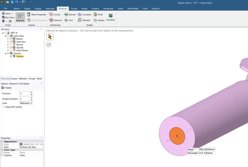
• Diameter of pipe

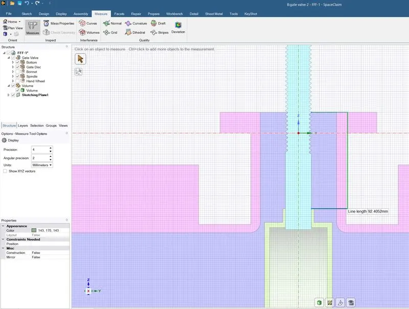
• Maximum Opening

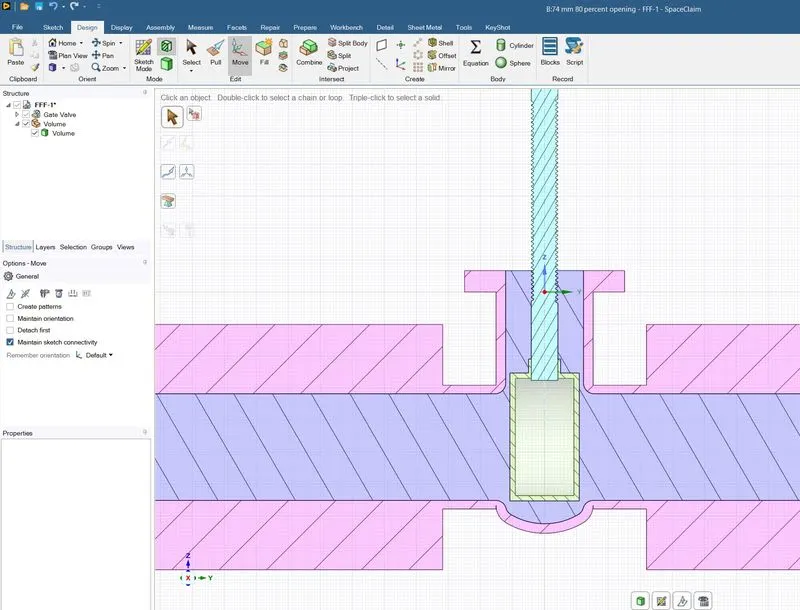
• 10% opening

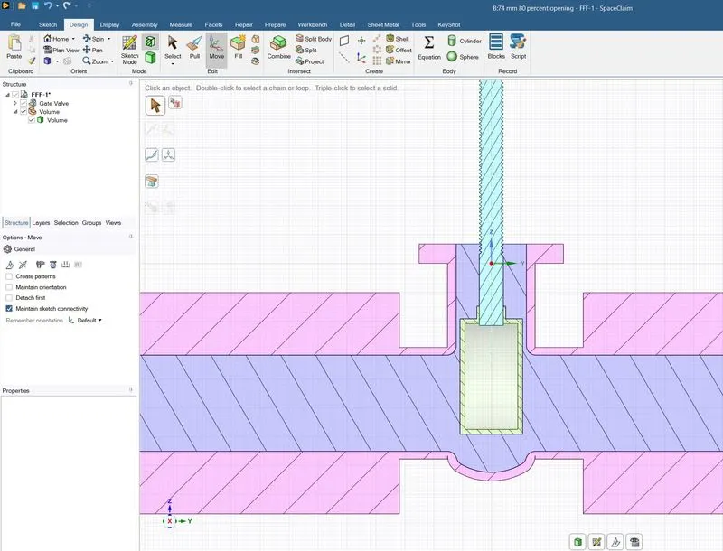
• 30% opening

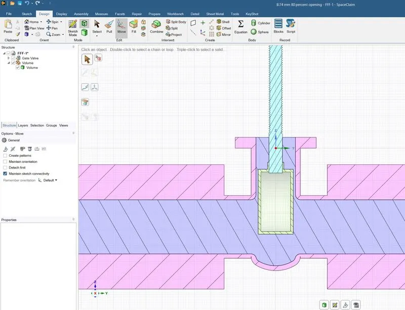
• 50% opening

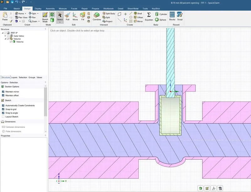
• 80% opening

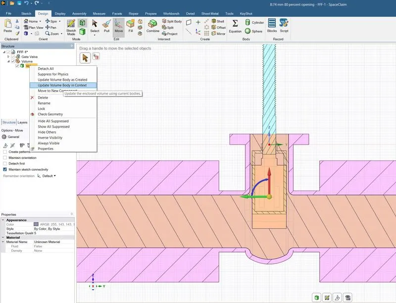
• Update disk movement

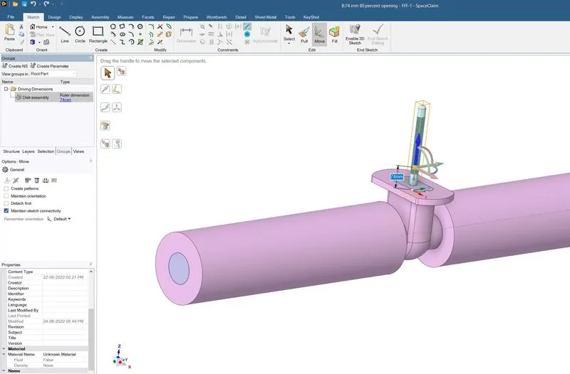
• Creating Parameters

Meshing:

• Meshing for this case is pretty straight forward, as we shall be generating mesh with a value of 10 mm as mesh size.
• Mesh generated is tetragonal in shape as this is a complex geometry.
• Although quality of mesh is not what is expected as per industry standard, the results are consistent. Reason for poor quality mesh is limitation of student version that doesn’t allow meshing of more than 500,000 cells.
• A lower size mesh will have cells more than half a million.
• Give Named Selections to input and outlet.

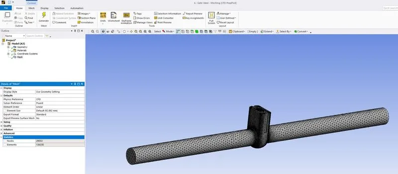
• Default mesh elements

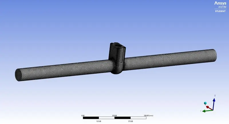
• 30% opening - Isometric View

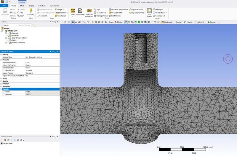
• 30% opening - Cut View

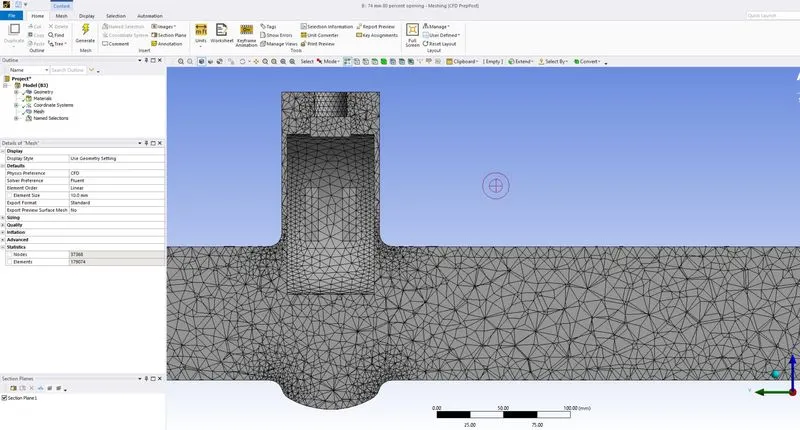
• refined mesh cut view - 80% opening

Setup:

Under setup, we perform the following steps.

• Once Fluent is loaded, we have various option under Outline View in left column.
• Under Setup tab in left column, click on General option, we get various options under Task Page. Ensure we have Pressure-Based type selected under Solver.
• Velocity formulation should be Absolute.
• Time advancement is Steady.
• Check Gravity, give in a value of -9.81 meter per squared second in negative Z direction.
• Next, Expand Models tab, Open Viscous model dialog box
• Choose k epsilon, Realizable model with Curvature correction and Production Limiter.
• Reason for checking these two options have been explained in ensuing paras.
• Expand Materials, right click on fluid and select new option. Add water-liquid as new material.
• Expand Cell zone Conditions, Fluid and open Volume. Change material from air to water.
• Go back to Fluids under materials and delete air.
• Under boundary conditions, change Inlet condition to pressure inlet from velocity inlet and give an inlet pressure of 10 Pascals.
• Leave the rest of options as is.
• Under Methods, choose coupled scheme as a pressure-velocity coupling as this is a steady state simulation.
• Change Turbulent kinetic energy and Dissipation Rate Discretization to second order upwind.
• Under initialization, Initialize from inlet.
• Once solution has been initialized, create contours after creating planes in YZ plane and other mass efflux report from outlet.
• Other reports can be generated as required. Our aim is to calculate area weighted average of pressure at inlet, mass efflux from the outlet.
• When creating mass efflux at outlet, click on create as an output parameter at the bottom of dialog box.
• Snippets for the same has been shown below.
• Run the simulation for about 200 iterations.

Curvature Correction for Two-Equation Models:

In order to sensitize to the effects of streamline curvature, a modification to the turbulence production term is available.

This is curvature correction option we get from the viscous model dialog box.

Production Limiters for Two-Equation Models:

A disadvantage of standard two-equation turbulence models is the excessive generation of the turbulence energy, GK, in the vicinity of stagnation points.

Stagnation points in our simulation is the region around gate disk. This is more pronounced in a 50 percent opening of gate disk.

In order to avoid the build-up of turbulent kinetic energy in the stagnation regions, production limiters are used.

This limiter does not affect the shear layer performance of the model, but avoids the stagnation point build-up.

By default, this limiter is enabled for all turbulence models based on the `\omega` equation.

Below images depict workflow in Fluent

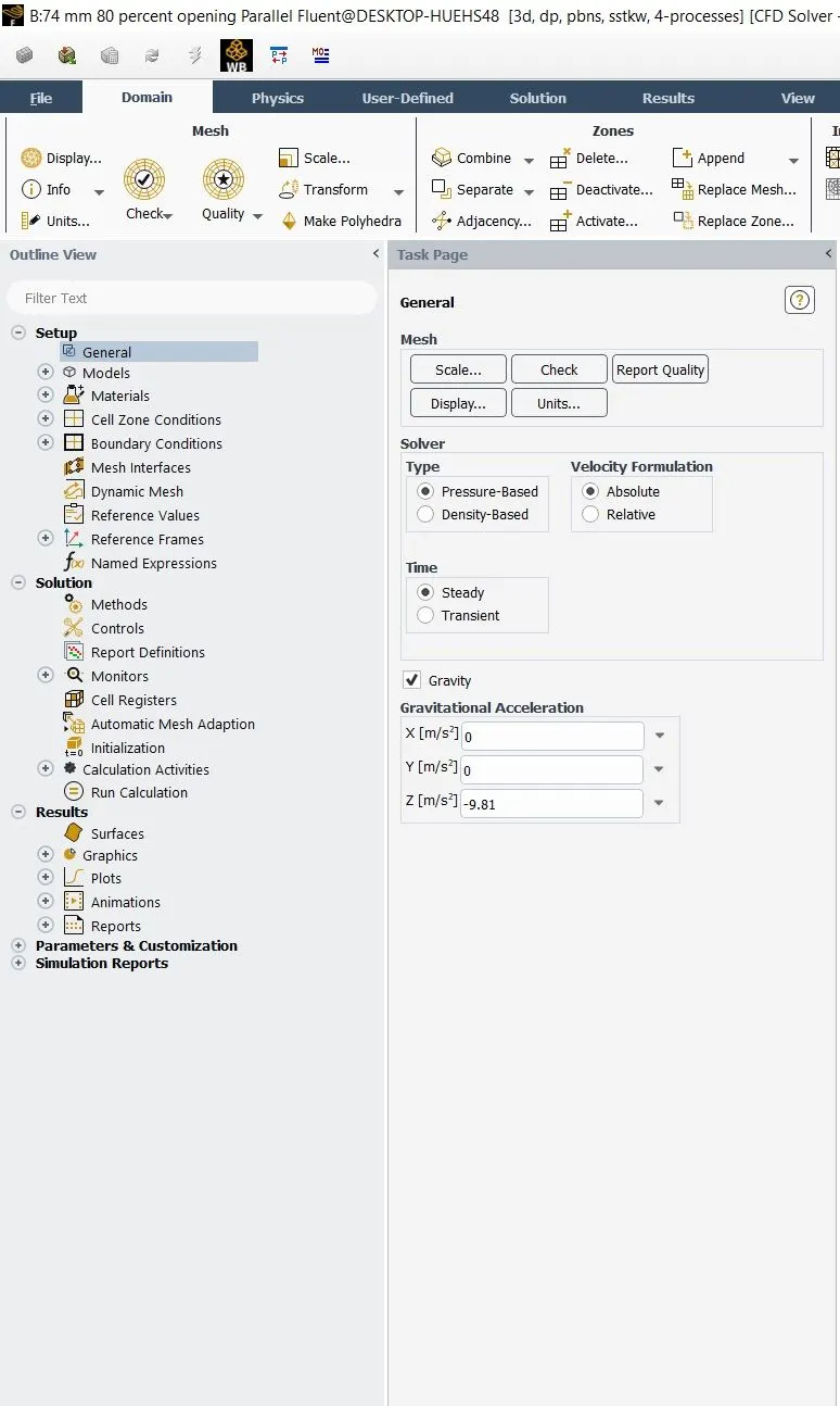
• General

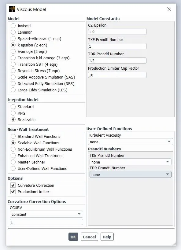
• Viscous model

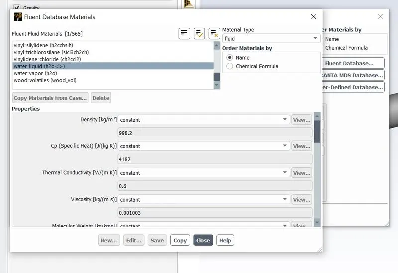
• add water

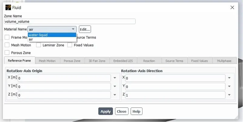
• change inner cells to water

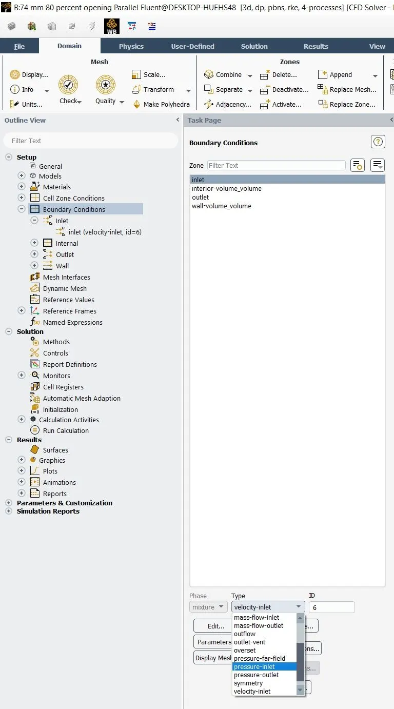
• Change velocity-inlet to pressure-inlet

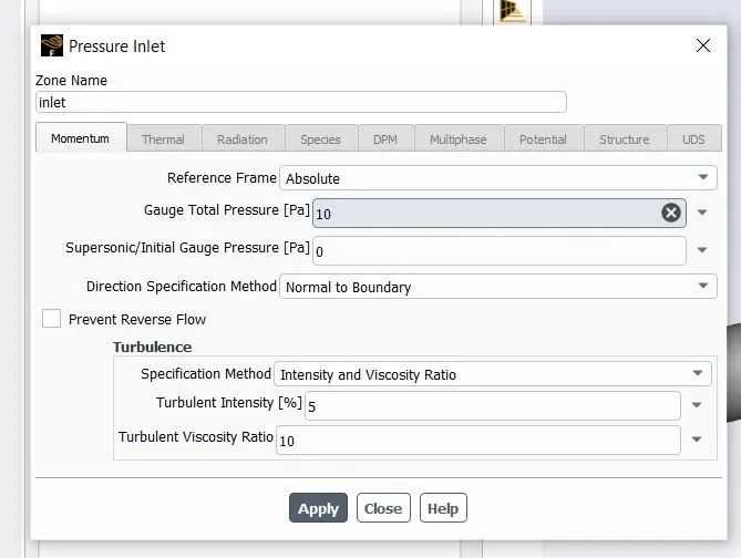
• inlet conditions

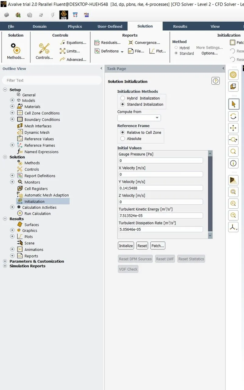
• Initialization

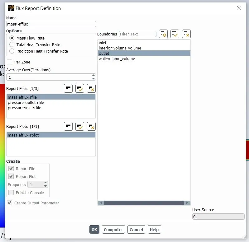
• Create flux report for parameters

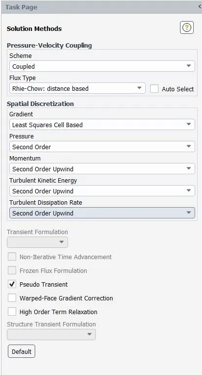
• Solution Methods

CFD-Post:

• Create a plane in YZ direction and create contour on the said plane for pressure and velocities.

RESULTS:

CASE 1 : 10% OPENING - 9.5 MM DISK LIFT

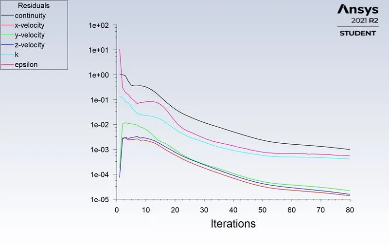
• Scaled Residuals

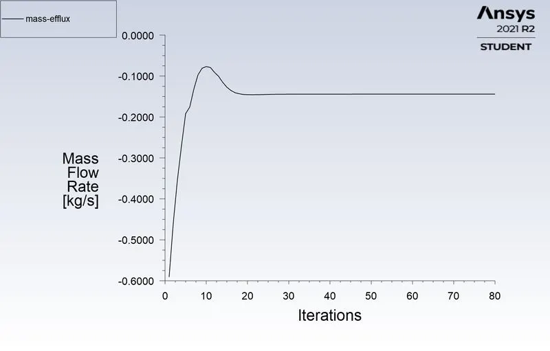
• mass efflux

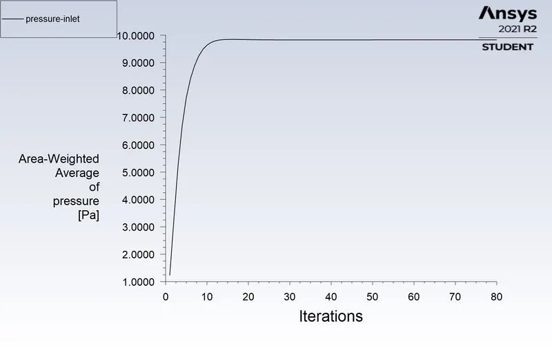
• pressure inlet

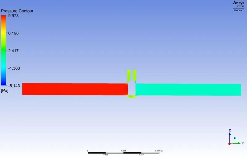
• Pressure Contour

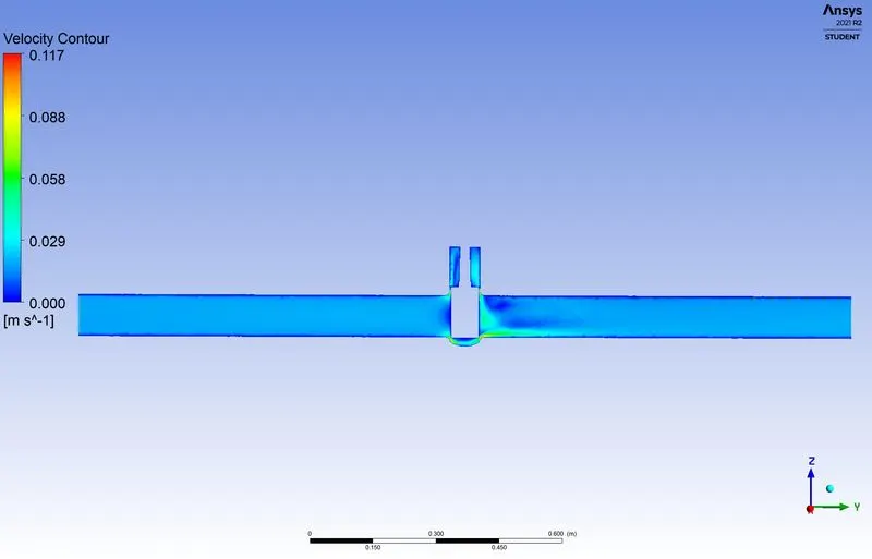
• Velocity Contour

CASE 2 : 30% OPENING - 27.8 MM DISK LIFT

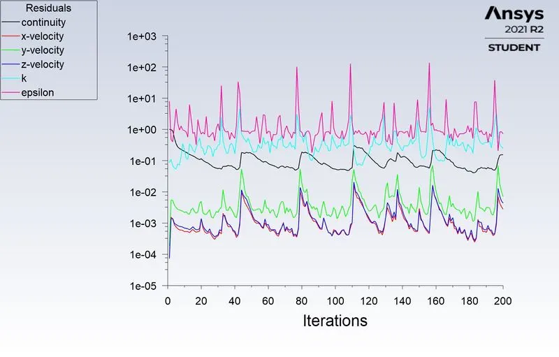
• Scaled Residuals

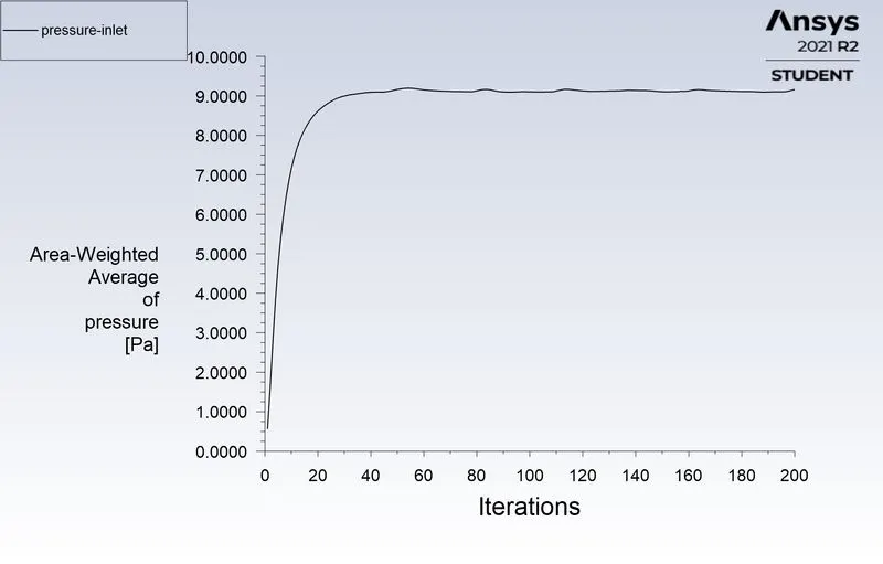
• Pressure Inlet

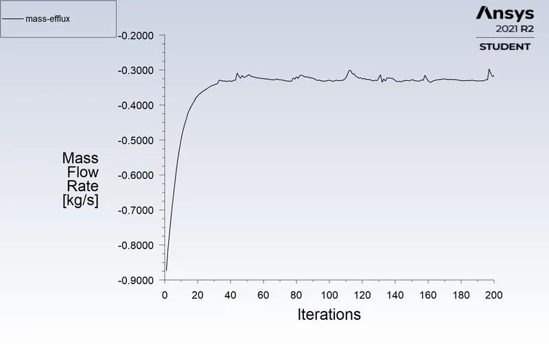
• Mass Efflux

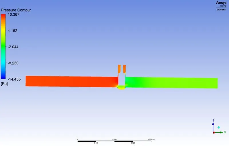
• Pressure Contour

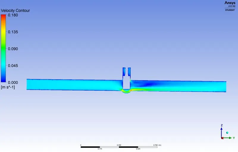
• Velocity Contour

CASE 3 : 50% OPENING - 46.5 MM DISK LIFT

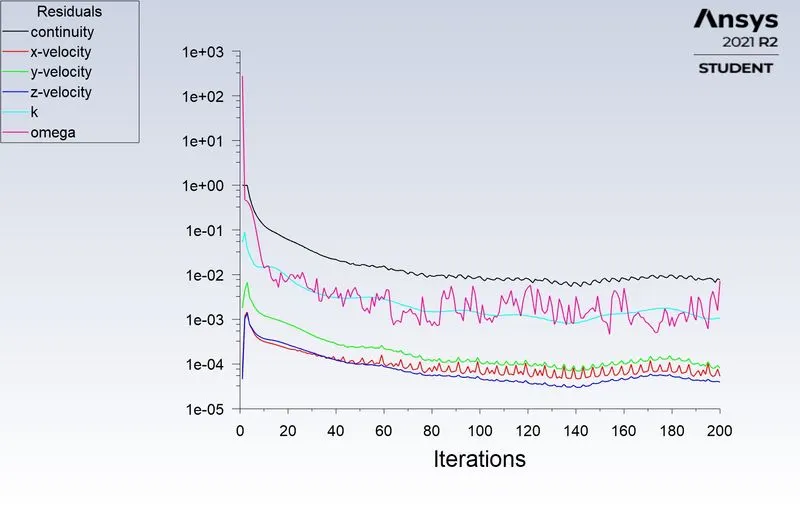
• Scaled Residuals using k omega model

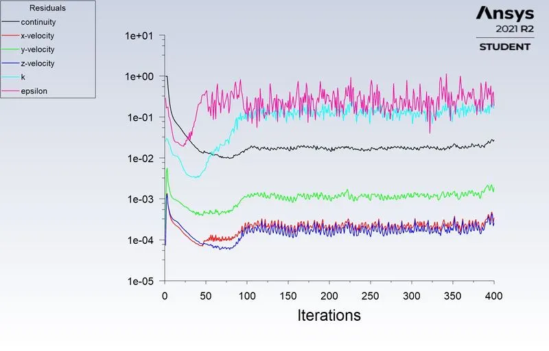
• Scaled residuals - scalable, curvature correction, production limiter

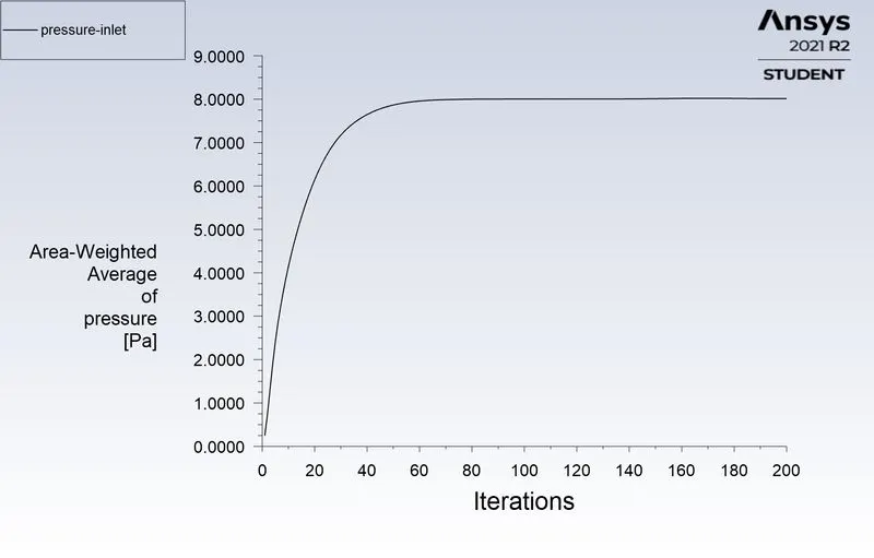
• Pressure Inlet

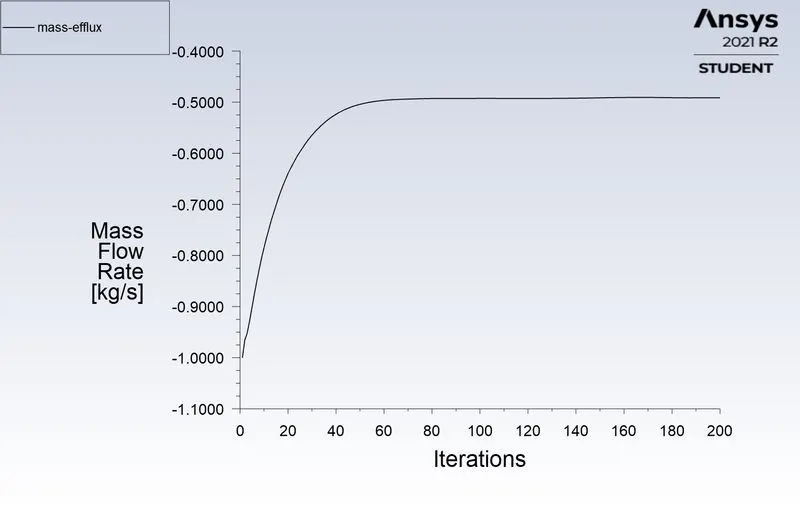
• Mass Efflux

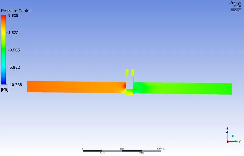
• Pressure Contour

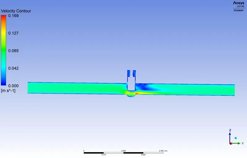
• Velocity Contour

CASE 4 : 80% OPENING - 74 MM DISK LIFT

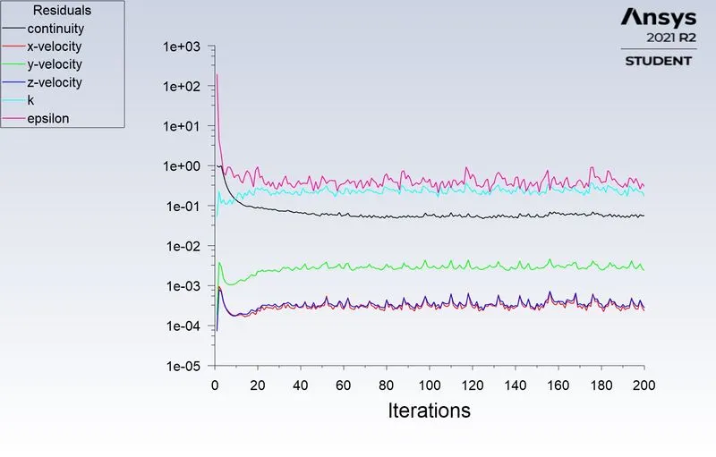
• Scaled Residuals

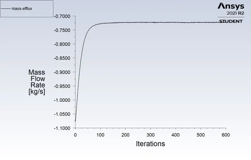
• Mass Efflux

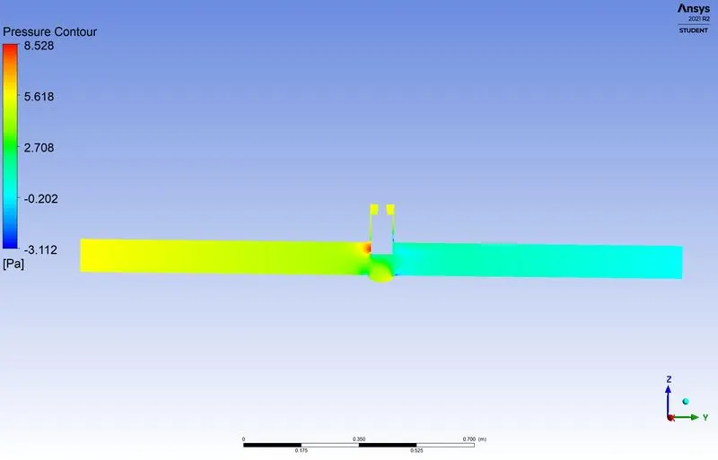
• Pressure Contour

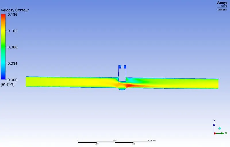
• Velocity Contour

Parameters:

• Under Disk assemble, add more options for various openings as discussed above and click on update against each of them.
• We have our mass efflux and pressure at inlets.

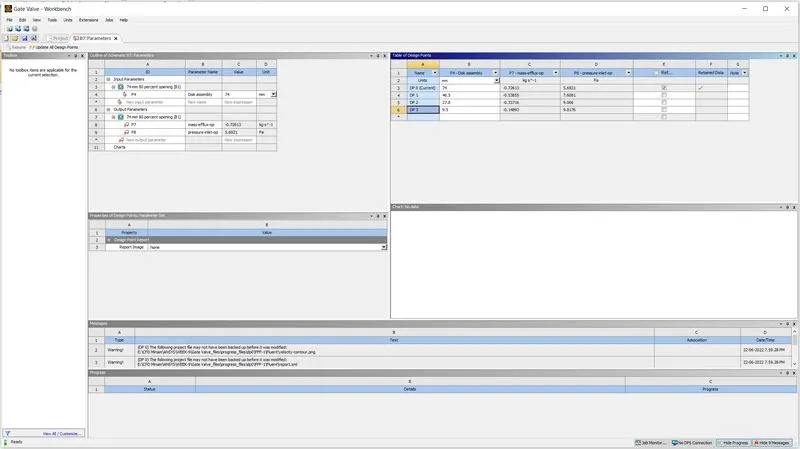
• Parameters Tab

• Table of Design Points

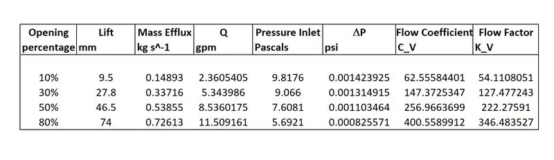
• Table of Cv and Kv

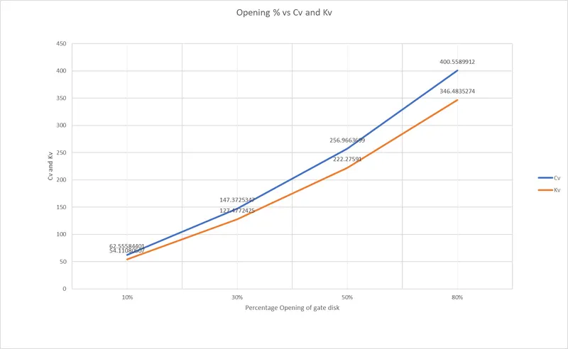
Conclusion:

• Mass flow rate increases with gradual increase in gate disc.
• As can be seen from the table, as gate disk opens up, the quantitative amount of water flowing through the disk also increases, this is flow coefficient expressed in gallons per minute. In SI units, the same is in cubic meters per hour and is called flow factor, which increases as well.
• Pressure in upstream of valve reduces as gate disk lift changes from fully shut to fully open.
• The k epsilon model for 50% lift of gate disk causes issues by not reaching an asymptotic value of mass efflux and pressure at inlet, this gives errors as solution to the same becomes iteration sensitive. This is because of non physical growth of turbulent generation at stagnation points around gate disk, in order to sensitize this issue, i.e; stabilize pseudo turbulent generation, a curvature correction term and production limiter was checked in viscous model dialog box.
• This project showcases various plots in results and from post-processing stages, these were done individually to validate the results obtained from parameters updates.
• These individual simulations run was not required and the output required for further studies can be set up by creating output parameters during parametrizing and taking the ensuing steps after running an update for the same.
• Thus, Parametric study reduces tedious and repetitive work by customizing specific parameters to be changed for simulating a seemingly large number of geometrically similar models.