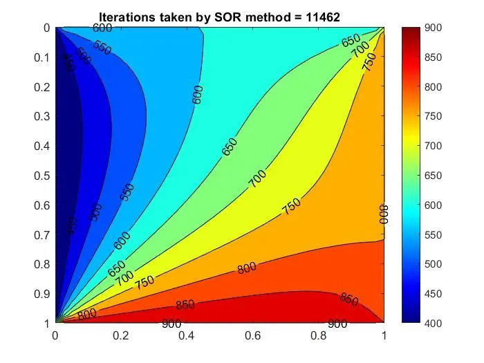
Week 5.1 - Mid term project - Solving the steady and unsteady 2D heat conduction problem
clear all
close all
clc

%% Define dimensions of the domain

L = 1;
% Nodes on each axis, only n is enough as uniform mesh is considered
n = 50;
% Define x and y array
x = linspace(0,1,n);
y = linspace(0,1,n);
% Size of mesh grid
dx = L/(n-1);
dy = dx;
% Define K as mesh grid in constant and does'nt change
K = ((2*(dx^2+dy^2)) / (dx^2*dy^2));

% Defining Boundary values into temperature array
T = nan(n,n);
% Assigning values to faces
West_face = 400;
East_face = 800;
North_face = 600;
South_face = 900;

% Defining Edges
T(2:end-1,1) = West_face;
T(2:end-1,end) =East_face;
T(1,2:end-1) = North_face;
T(end,2:end-1) = South_face;

% Defining Corners
T(1,1) = (North_face+West_face)/2;
T(end,1) = (South_face+West_face)/2;
T(1,end) = (North_face+East_face)/2;
T(end,end) = (South_face+East_face)/2;

% Assuming initial values to the temperature array
T(2:end-1,2:end-1) = 150;

% Assign array to another array for each method
T_old = T;
T_gs_updated = T;
T_gs2 = T;
T_SOR_updated = T;
T_SOR = T;

%% Steady 2D Diffusion Problem - Jacobi Method


tolerance = 1e-4;
jakobi_iterations = 1;
abs_error = 1e5;

tic
while (abs_error > tolerance)
    for i = 2:n-1 % Traversing rows
        for j = 2:n-1 % Traversing columns

            T_E = T_old(i,j+1);T_W = T_old(i,j-1);
            T_N = T_old(i-1,j);T_S = T_old(i+1,j);
            T(i,j) = ((1/K) * (T_E+T_W)/dx^2 ) + ((1/K) * (T_N+T_S)/dy^2 );

        end
    end

    abs_error = max(max(abs(T-T_old)));
    T_old = T;
    jakobi_iterations = jakobi_iterations+1;

end
jakobi_sim_time = toc;

fprintf('Computational time using Jakobi Solver = %.3f\n',jakobi_sim_time)
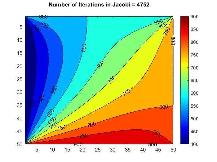
fprintf('Number of Iterations = %g\n',jakobi_iterations)

% Give contour & fill with colours
[c,d] = contourf(T);
% Give colormap Name as hsv, from doc 'colormap'
colormap jet
% Define color bar to the right of plot for temp reference
colorbar
clabel(c,d)
% Mirror plot about x axis to imitate top and bottom boundary conditions
% from the domain
H = gca;
set(H,'YDir','reverse')
title(sprintf('Number of Iterations in Jakobi = %g\n',jakobi_iterations))


%% Steady 2D Diffusion Problem - Gauss-Seidel Method

GS_iterations = 1;
abs_error = 1e5;

tic
while (abs_error > tolerance)
    for i = 2:n-1 % Traversing rows
        for j = 2:n-1 % Traversing columns

            % Since I am traversing the columns, I know my north and west
            % values of each node & need to be updated
            T_E = T_gs2(i,j+1);T_W = T_gs_updated(i,j-1);
            T_N = T_gs_updated(i-1,j);T_S = T_gs2(i+1,j);
            T_gs_updated(i,j) = ((1/K) * (T_E+T_W)/dx^2) + ((1/K) * (T_N+T_S)/dy^2);

        end
    end

    abs_error = max(max(abs(T_gs_updated - T_gs2)));
    T_gs2 = T_gs_updated;
    GS_iterations = GS_iterations+1;

end
GS_sim_time = toc;

fprintf('Computational time using Gauss-Seidel Solver = %.3f\n',GS_sim_time)
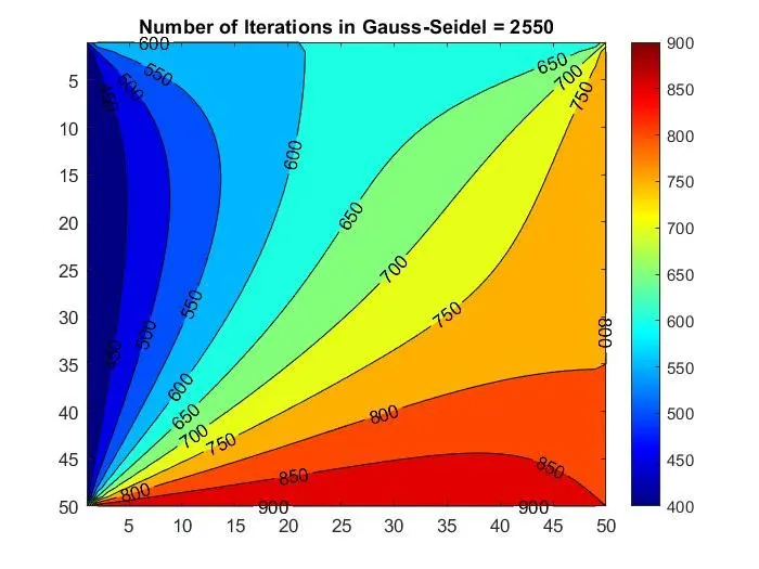
fprintf('Number of Iterations = %g\n',GS_iterations)

figure
% Give contour & fill with colours
[c,d] = contourf(T_gs2);
% Give colormap Name as hsv, from doc 'colormap'
colormap jet
% Define color bar to the right of plot for temp reference
colorbar
clabel(c,d)
% Mirror plot about x axis to imitate top and bottom boundary conditions
% from the domain
H = gca;
set(H,'YDir','reverse')
title(sprintf('Number of Iterations in Gauss-Seidel = %g',GS_iterations))


%% Steady 2D Diffusion Problem - Successive Over Relaxation Method

SOR_iterations = 1;
abs_error = 1e5;
alpha = 1.4;

tic
while (abs_error > tolerance)
    for i = 2:n-1 % Traversing rows
        for j = 2:n-1 % Traversing columns

            T_E = T_SOR(i,j+1);T_W = T_SOR_updated(i,j-1);
            T_N = T_SOR_updated(i-1,j);T_S = T_SOR(i+1,j);
            T_SOR_updated(i,j) = ((1/K) * (T_E+T_W)/dx^2) + ((1/K) * (T_N+T_S)/dy^2);
            T_SOR_updated(i,j) = (alpha * T_SOR_updated(i,j)) + ((1-alpha)*T_SOR(i,j));


        end
    end

    abs_error = max(max(abs(T_SOR_updated - T_SOR)));
    T_SOR = T_SOR_updated;
    SOR_iterations = SOR_iterations + 1;

end
SOR_sim_time = toc;

fprintf('Computational time using SOR Solver = %.3f\n',GS_sim_time)
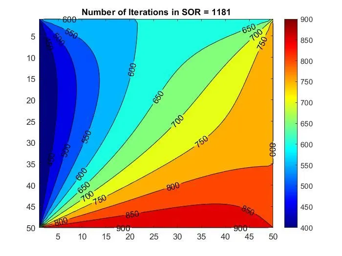
fprintf('Number of Iterations = %g\n',SOR_iterations)

figure
% Give contour & fill with colours
[c,d] = contourf(T_SOR);
% Give colormap Name as hsv, from doc 'colormap'
colormap jet
% Define color bar to the right of plot for temp reference
colorbar
clabel(c,d)
% Mirror plot about x axis to imitate top and bottom boundary conditions
% from the domain
H = gca;
set(H,'YDir','reverse')
title(sprintf('Number of Iterations in SOR = %g',SOR_iterations))

================ END OF PROGRAM 1 PLEASE RUN THE BELOW SCRIPT SEPARATELY ============

clear all
close all
clc

%% Define dimensions of the domain

L = 1;
% Nodes on each axis, only n is enough as uniform mesh is considered
n = 40;
% Define x and y array
x = linspace(0,1,n);
y = linspace(0,1,n);
% Size of mesh grid
dx = L/(n-1);
dy = dx;

% Defining Boundary values into temperature array
T = ones(n,n);
% Assigning values to faces
West_face = 400;
East_face = 800;
North_face = 600;
South_face = 900;

% Defining Edges
T(2:end-1,1) = West_face;
T(2:end-1,end) =East_face;
T(1,2:end-1) = North_face;
T(end,2:end-1) = South_face;

% Defining Corners
T(1,1) = (North_face+West_face)/2;
T(end,1) = (South_face+West_face)/2;
T(1,end) = (North_face+East_face)/2;
T(end,end) = (South_face+East_face)/2;

% Assuming initial values to the temperature array
T(2:end-1,2:end-1) = 150;

% Assign array to another array for each method
T_old = T;
T_new = T;

% Defining standard constants k1 k2 and alpha
alpha = 1.4;
dt = 0.0001;
k1 = alpha*dt/(dx^2);
k2 = alpha*dt/(dy^2);
end_time = 0.4;
% number of time steps
nt = end_time / dt;

% This value should be less than 0.5 for convergence to occur
check = k1+k2;

%% Unsteady (Explicit Scheme) 2D Diffusion Problem

iterations = 1;
tic
for it = 1:nt
     for i = 2:n-1 % Traversing rows
         for j = 2:n-1 % Traversing columns

                T_E = T_old(i,j+1);T_W = T_old(i,j-1);
                T_N = T_old(i-1,j);T_S = T_old(i+1,j);
                term_1 = (T_old(i,j)*(1-(2*k1)-(2*k2)));
                term_2 = (k1*(T_E + T_W));
                term_3 = (k2*(T_N+T_S));

                T_new(i,j) = term_1+term_2+term_3;
        end
     end
    T_old = T_new;
    iterations = iterations+1;
end

Explicit_Sim_time = toc;

fprintf('Computational time for Explicit Scheme = %.3f\n',Explicit_Sim_time)
fprintf('Number of Iterations = %g\n',iterations)

% Give contour & fill with colours
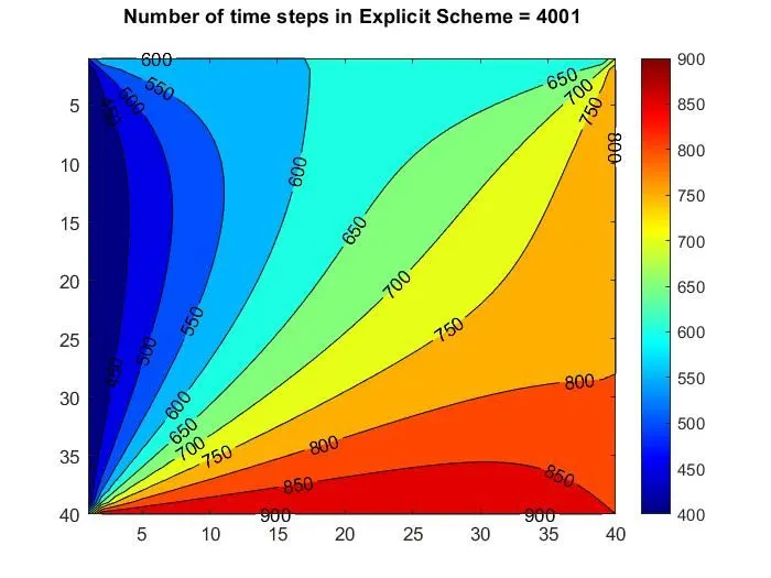
[c,d] = contourf(T_new);
% Give colormap Name as hsv, from doc 'colormap'
colormap jet
% Define color bar to the right of plot for temp reference
colorbar
clabel(c,d)
% Mirror plot about x axis to imitate top and bottom boundary conditions
% from the domain
H = gca;
set(H,'YDir','reverse')
title(sprintf('Number of time steps in Explicit Scheme = %g\n',iterations))

================ END OF PROGRAM 1 PLEASE RUN THE BELOW SCRIPT SEPARATELY ============

clear all
close all
clc

%% Define dimensions of the domain

L = 1;
% Nodes on each axis, only n is enough as uniform mesh is considered
n = 40;
% Define x and y array
x = linspace(0,1,n);
y = linspace(0,1,n);
[xx,yy] = meshgrid(x,y);
% Size of mesh grid
dx = L/(n-1);
dy = dx;

% Defining Boundary values into temperature array
T = ones(n,n);
% Assigning values to faces
West_face = 400;
East_face = 800;
North_face = 600;
South_face = 900;

% Defining Edges
T(2:end-1,1) = West_face;
T(2:end-1,end) =East_face;
T(1,2:end-1) = North_face;
T(end,2:end-1) = South_face;

% Defining Corners
T(1,1) = (North_face+West_face)/2;
T(end,1) = (South_face+West_face)/2;
T(1,end) = (North_face+East_face)/2;
T(end,end) = (South_face+East_face)/2;

% Assuming initial values to the temperature array
T(2:end-1,2:end-1) = 150;

% Assign array to another array for each method
T_old = T;
T_prev_dt1 = T;
T_prev_dt2 = T;
T_prev_dt3 = T;
T_gs = T;
T_gs_updated = T;
T_sor = T;
T_sor_updated = T;

% Defining standard constants k1 k2 and alpha
alpha = 1.5;
dt = 0.0001;
k1 = alpha*dt/(dx^2);
k2 = alpha*dt/(dy^2);

% This value should be less than 0.5 for convergence to occur
check = k1+k2;

term1 = (1+(2*k1)+(2*k2))^-1;
term2 = k1*term1;
term3 = k2*term1;

tolerance = 1e-4;


%% Unsteady (Implicit Scheme) 2D Diffusion Problem - Jacobi Method

count_J=1;
tic
for it = 1:1400
    error = 1e9;
    while error > tolerance % Convergence loop
        % Spacial loop
     for i = 2:n-1   % Traversing the rows
         for j=2:n-1  % Traversing the columns
             H = T_old(i,j-1) + T_old(i,j+1);
             V = T_old(i-1,j) + T_old(i+1,j);
             T(i,j) = (T_prev_dt1(i,j)*term1) + (term2*H) + (term3*V);
         end
     end
     error = max(max(abs(T-T_old)));
     T_old = T;
     count_J=count_J+1;
    end
    % Go to the next time step
    T_prev_dt1 = T;
    [c,d] = contourf(xx,yy,T,'ShowText','on');
    hold on
    set(gca,'YDir','reverse')
    colorbar
    colormap jet
    pause(0.00001)
    clabel(c,d)
    hold off
end
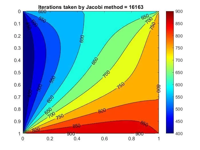
title(sprintf('Iterations taken by Jacobi method = %d',count_J))

Jacobi_sim_time = toc;

%% Unsteady (Implicit Scheme) 2D Diffusion Problem - Gauss-Seidel Method

count_GS=1;
tic
figure(2)
for it = 1:1400
    error = 1e9;
    while error > tolerance % Convergence loop
        % Space loop
     for i = 2:n-1   % Traversing the rows
         for j=2:n-1  % Traversing the columns
             H = T_gs_updated(i,j-1) + T_gs(i,j+1);
             V = T_gs_updated(i-1,j) + T_gs(i+1,j);
             T_gs_updated(i,j) = (T_prev_dt2(i,j)*term1) + (term2*H) + (term3*V);
         end
     end
     error = max(max(abs(T_gs-T_gs_updated)));
     T_gs = T_gs_updated;
     count_GS=count_GS+1;
    end
    % Go to the next time step
    T_prev_dt2 = T_gs_updated;
    [c,d] = contourf(xx,yy,T_gs,'ShowText','on');
    set(gca,'YDir','reverse')
    colorbar
    colormap jet
    pause(0.00001)
    clabel(c,d)

end
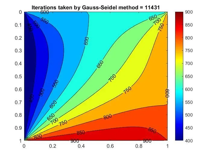
title(sprintf('Iterations taken by Gauss-Seidel method = %d',count_GS))

GS_sim_time = toc;

%% Unsteady (Implicit Scheme) 2D Diffusion Problem - SOR Method

count_SOR=1;
omega = 1.005;
tic
figure(3)
for it = 1:1400
    error = 1e9;
    while error > tolerance % Convergence loop
        % Spacial loop
     for i = 2:n-1   % Traversing the rows
         for j=2:n-1  % Traversing the columns
             H = T_sor_updated(i,j-1) + T_sor(i,j+1);
             V = T_sor_updated(i-1,j) + T_sor(i+1,j);
             T_sor_updated(i,j) = (T_prev_dt3(i,j)*term1) + (term2*H) + (term3*V);
             T_sor_updated(i,j) = omega*T_sor_updated(i,j) + ((1-omega)*T_prev_dt3(i,j));
         end
     end
     error = max(max(abs(T_sor-T_sor_updated)));
     T_sor = T_sor_updated;
     count_SOR = count_SOR+1;
    end
    % Go to the next time step
    T_prev_dt3 = T_sor_updated;
    [c,d] = contourf(xx,yy,T_sor,'ShowText','on');
    set(gca,'YDir','reverse')
    colorbar
    colormap jet
    pause(0.00001)
    clabel(c,d)
end
title(sprintf('Iterations taken by SOR method = %d',count_SOR))

SOR_sim_time = toc;
IMPORTANT NOTE:
There are three scripts in the code above, that need to be run SEPARATELY. After Every script, It shows end of Program 1, Please rub the below script Separately!
Attaching plots below.
- Steady 2D Diffusion Jacobi Iterative Method
- Steady 2D Diffusion Gauss-Seidel Iterative Method
-
- Steady 2D Diffusion SOR Iterative Method
- Un-Steady diffusion Explicit method
- Unsteady (Implicit) 2D Diffusion - Jacobi method
- Unsteady (Implicit) 2D Diffusion - Gauss-Seidel method
- Unsteady (Implicit) 2D Diffusion - SOR method