Week 11 - Simulation of Flow through a pipe in OpenFoam
Week 11 - Simulation of Flow through a pipe in OpenFoam
In this challenge, we shall simulate an axi-symmetric flow by applying a wedge boundary condition.
Problem Statement:
- The flow is axi-symmetric.
- Wedge Boundary condition is used.
- Flow is laminar and flows through a constant cross section pipe.
- Reynolds number is 2100.
- A transient or steady state solution can be used to obtain the results.
- Use MATLAB to generate BlockMeshDict file.
Results recorded in this report:
- Validating hydro-Dynamic length with Numerical results
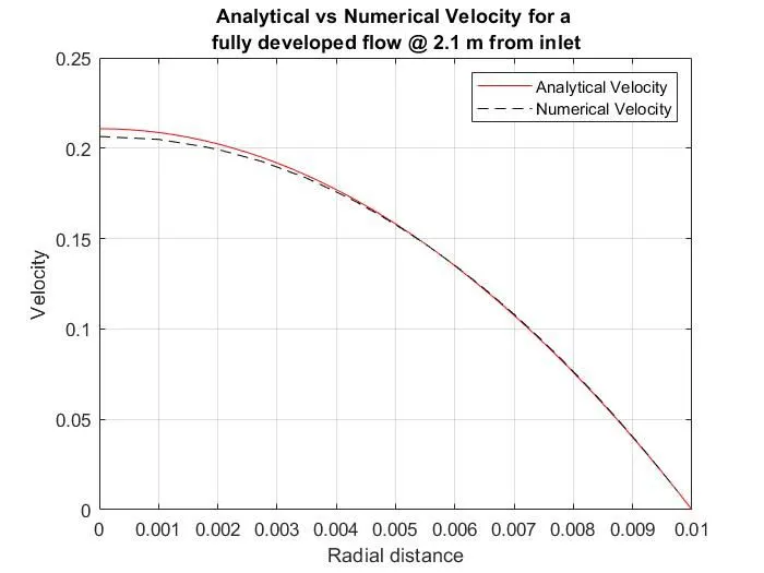
- Validating fully developed flow velocity profile with its analytical profile
- Validating pressure drop for fully developed flow
- Post-process shear stress and validate wall shear stress for fully developed flow.
Wedge type boundary:
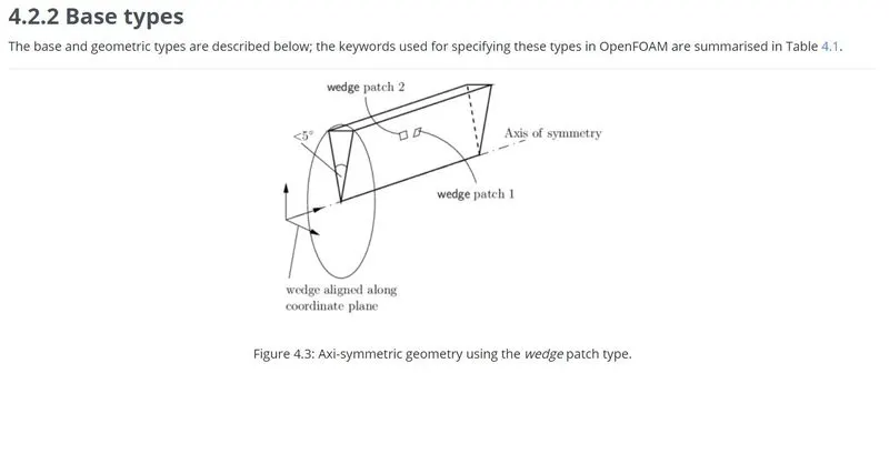
Before we start with the actual report, we need to understand what an axi-symmetric flow is;
An axi-symmetry flow is one in which the streamlines are symmetrically located around the axis. Every longitudinal plane through the axis would exhibit the same streamline pattern.
Properties of the fluid considered in this report are thus;
- Working Fluid: Water @ 25 C
- Dynamic Viscosity: 1.002e-03 Ns/m2
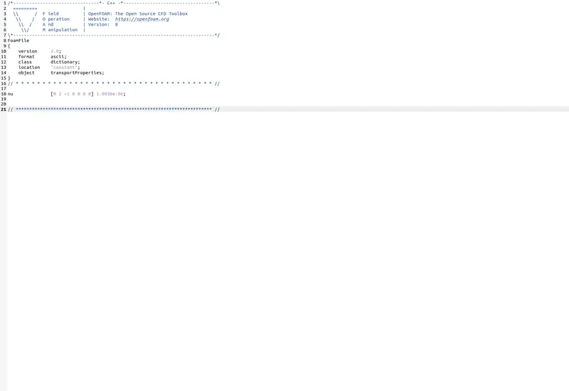
- Kinematic Viscosity: 1.0038e-06 (m/s)2
- Density: 998.21 kg/m3
Analytical Formulas used in Hagen Poiseuille flow:
- Velocity at any radial location:
`V_r=R^2/(4μ) ((dp)/dz)(1-(r^2/R^2 ))`
At the pipe centre, r=0; this gives us a maximum velocity. Substituting r=0 in the above equation, we get;
`V_max=R^2/(4μ) ((dp)/dx)`
As per Hagen Poiseuille analysis for a pipe, in the fully developed flow region, for a laminar flow, the velocity profile is parabolic in nature and the velocity distribution is as given above.
Thus, our original equation becomes
`V_r=V_max (1-(r^2/R^2 ))`
Velocity at the axis is maximum, thus;
`(dV_r)/(dr)=0` at axis
The derivative as shown above, when applied to the Vr equation, yields us the maximum velocity in terms of average velocity which is given by;
`V_max=2.V_(avg)` m/s
Formula for Reynolds number calculation; Dimensionless
`Re=(ρU_(avg) D)/μ`
Pressure-drop using Hagen Poiseuille equation:
`∆P=(32μU_(avg) L)/D^2` Pascals
Steps to be followed to perform calculations:
- Since the flow is laminar in nature, we know for a pipe, flow shall remain laminar when Reynolds number is less than 2200. We shall thus consider a flow with Reynolds number 2100 as given in the problem statement.
- Density and dynamic viscosity are known from standard tables (a number of sources on the internet will give the standard values)
- Based on these, the average velocity can be now calculated.
- Maximum Velocity is twice the average velocity.
Choosing the Diameter:
Entrance length: The length from the inlet at which a fully developed velocity profile is attained.
The empirical formula from literature, for the entrance length is given as
`L/D=0.05*Re`
We shall choose a diameter of 2 cm, as larger diameter for given Reynolds number of 2100, would result in a velocity of very low magnitude which would traverse the entire length of the pipe taking more time. To reduce the total time of simulation, we decide to go with a value of 2 cm for the diameter.
The entrance length we get using the given values is about 2.1 meters. We can round the total length of pipe to 3 meters.
Average Velocity:
Based on this value, we get an average velocity of 0.1054 m/s.
The maximum velocity then is 0.2108 m/s.
Pressure Drop:
Pressure-drop, using the formula given above, gives us a value of 25.3463 Pascals. This, when divided by the density would give us a value of 0.0254 (m/s)2.
A snippet of the MATLAB code which performs and yields the above analytical values is shown below.
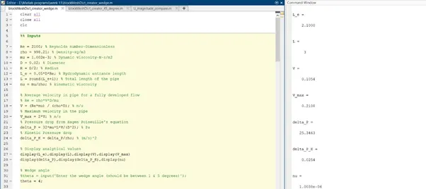
We now, using MATLAB program, create a blockMeshDict file in .txt format.
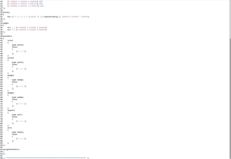
The Script and resulting .txt file are shown below.
clear all
close all
clc

%% Inputs

Re = 2100; % Reynolds number-Dimensionless
rho = 998.21; % Density-kg/m3
mu = 1.002e-3; % Dynamic viscosity-N-s/m2
D = 0.02; % Diameter
R = D/2; % Radius
L_e = 0.05*D*Re; % Hydrodynamic entrance length
L = round(L_e+1); % Total length of the pipe
nu = mu/rho; % kinematic viscosity

% Average velocity in pipe for a fully developed flow
% Re = rho*V*D/mu
V = (Re*mu) / (rho*D); % m/s
% Maximum velocity in the pipe
V_max = 2*V; % m/s
% Pressure drop from Hagen Poiseuille's equation
delta_P = 32*mu*L*V/(D^2); % Pa
% Kinetic Pressure drop
delta_P_K = delta_P/rho; % (m/s)^2

% Display analytical values
display(L_e),display(L),display(V),display(V_max)
display(delta_P),display(delta_P_K),display(nu)

% Wedge angle
%theta = input('Enter the wedge angle (should be between 1 & 5 degrees)');
theta = 4;

% Meshing
mesh_x = 200;
mesh_y = 20;
mesh_z = 1;

% Mesh grading factors
grade_x = 1;
grade_y = 0.2;
grade_z = 1;

% Defining various blank sizes
b1 = blanks(4);
b2 = blanks(8);
b3 = blanks(12);


%% Calculating magnitude of vertices

v_0 = [0 0 0];
v_1 = [0 R*cosd(theta/2) R*sind(theta/2)]; %1 is right of centreline
v_2 = [0 R*cosd(theta/2) -R*sind(theta/2)];
v_3 = [L 0 0];
v_4 = [L R*cosd(theta/2) R*sind(theta/2)];
v_5 = [L R*cosd(theta/2) -R*sind(theta/2)];


%% Creating BlockMeshDict file

h1 = '/*--------------------------------*- C++ -*----------------------------------*\';
h2 = '  =========                 |';
h3 = '  \\      /  F ield         | OpenFOAM: The Open Source CFD Toolbox';
h4 = '   \\    /   O peration     | Website:  https://openfoam.org';
h5 = '    \\  /    A nd           | Version:  8';
h6 = '     \\/     M anipulation  |';
h7 = '\*---------------------------------------------------------------------------*/';
h8 = 'FoamFile';
h9 = '// * * * * * * * * * * * * * * * * * * * * * * * * * * * * * * * * * * * * * //';
h_end = '// ************************************************************************* //';

% Create and open blockmesh file
f1 = fopen('blockMeshDict.txt','w');

% Creating header
fprintf(f1,'%s\n',h1);
fprintf(f1,'%s\n',h2);
fprintf(f1,'%s\n',h3);
fprintf(f1,'%s\n',h4);
fprintf(f1,'%s\n',h5);
fprintf(f1,'%s\n',h6);
fprintf(f1,'%s\n',h7);
fprintf(f1,'%s\n',h8);
fprintf(f1,'{\n');
fprintf(f1,'%s\n','    version     2.0;');
fprintf(f1,'%s\n','    format      ascii;');
fprintf(f1,'%s\n','    class       dictionary;');
fprintf(f1,'%s\n','    object      blockMeshDict;');
fprintf(f1,'}\n');
fprintf(f1,'%s\n\n',h9);
fprintf(f1,'convertToMeters 1;\n\n');

%% Defining the Vertices

% Opening Statement
fprintf(f1,'vertices\n(\n');
% vertex 0
fprintf(f1,'%s(%d %d %d) //0\n',b1,v_0(1),v_0(2),v_0(3));
% vertex 1
fprintf(f1,'%s(%f %f %f) //1\n',b1,v_1(1),v_1(2),v_1(3));
% vertex 2
fprintf(f1,'%s(%f %f %f) //2\n',b1,v_2(1),v_2(2),v_2(3));
% vertex 3
fprintf(f1,'%s(%f %f %f) //3\n',b1,v_3(1),v_3(2),v_3(3));
% vertex 4
fprintf(f1,'%s(%f %f %f) //4\n',b1,v_4(1),v_4(2),v_4(3));
% vertex 5
fprintf(f1,'%s(%f %f %f) //5\n',b1,v_5(1),v_5(2),v_5(3));
% Closing Statement
fprintf(f1,');\n\n');

%% Defining Blocks and Edges

% Block
% Opening Statement
fprintf(f1,'blocks\n(\n');
fprintf(f1,'%shex (0 3 5 2 0 3 4 1) ',b1);
fprintf(f1,'(%d %d %d) ',mesh_x,mesh_y,mesh_z);
fprintf(f1,'simpleGrading (%f %f %f)',grade_x,grade_y,grade_z);
% Closing Statement
fprintf(f1,'\n);\n\n');
% Edges
fprintf(f1,'edges\n(\n');
fprintf(f1,'%sarc 1 2 (%f %f %f)\n',b1,0,R,0);
fprintf(f1,'%sarc 4 5 (%f %f %f)\n',b1,L,R,0);
fprintf(f1,');\n\n');

%% Defining Boundaries

inflow = [0 1 2 0];
outflow = [3 5 4 3];
wedge_1 = [0 2 5 3]; % back
wedge_2 = [0 3 4 1]; % front
noslipwalls = [1 4 5 2];
axis = [0 3 3 0];

% Inlet
fprintf(f1,'boundary\n(\n');
fprintf(f1,'%sinlet\n%s{\n',b1,b1);
fprintf(f1,'%stype patch;\n',b2);
fprintf(f1,'%sfaces\n%s(\n',b2,b2);
fprintf(f1,'%s(%d %d %d %d)\n',b3,inflow);
fprintf(f1,'%s);\n%s}\n',b2,b1);

% Outlet
fprintf(f1,'%soutlet\n%s{\n',b1,b1);
fprintf(f1,'%stype patch;\n',b2);
fprintf(f1,'%sfaces\n%s(\n',b2,b2);
fprintf(f1,'%s(%d %d %d %d)\n',b3,outflow);
fprintf(f1,'%s);\n%s}\n',b2,b1);

% wedge-1 and 2
fprintf(f1,'%swedge1\n%s{\n',b1,b1);
fprintf(f1,'%stype wedge;\n%sfaces\n%s(\n',b2,b2,b2);
fprintf(f1,'%s(%d %d %d %d) %s\n',b3,wedge_1,'// Wedge-1');
fprintf(f1,'%s);\n%s}\n',b2,b1);

% wedge-2
fprintf(f1,'%swedge2\n%s{\n',b1,b1);
fprintf(f1,'%stype wedge;\n%sfaces\n%s(\n',b2,b2,b2);
fprintf(f1,'%s(%d %d %d %d) %s\n',b3,wedge_2,'// Wedge-2');
fprintf(f1,'%s);\n%s}\n',b2,b1);

% noslipwalls
fprintf(f1,'%stopwall\n%s{\n',b1,b1);
fprintf(f1,'%stype wall;\n%sfaces\n%s(\n',b2,b2,b2);
fprintf(f1,'%s(%d %d %d %d)\n',b3,noslipwalls);
fprintf(f1,'%s);\n%s}\n',b2,b1);

% Define the axis
fprintf(f1,'%saxis\n%s{\n',b1,b1);
fprintf(f1,'%stype empty;\n%sfaces\n%s(\n',b2,b2,b2);
fprintf(f1,'%s(%d %d %d %d)\n',b3,axis);
fprintf(f1,'%s);\n%s}\n);\n\n',b2,b1);

% mergePatchPairs
fprintf(f1,'mergePatchPairs\n(\n);\n\n');
fprintf(f1,'%s\n',h_end);

%% Numerical values extracted from OpenFOAM

V_0 = xlsread('U @ 2.1 m from inlet_40points.csv');
V_rnum = V_0(1:end,1);

%% Fully developed flow velocity profile - Analytical

r = linspace(0,R,41);
[V_r] = V_max*(1-(r.^2./R^2)); % Analytical values

%% Plotting a graph for Velocity vs Radial distance

plot(r,V_r,'r',r,V_rnum,'k--')
xlabel('Radial distance')
ylabel('Velocity')
legend('Analytical Velocity','Numerical Velocity')
grid on
title({'Analytical vs Numerical Velocity for a ';'fully developed flow @ 2.1 m from inlet'})

%% Calculating the error

error = nan(1,length(r));

for i = 1:length(V_r)
    if gt(V_r(i),V_rnum(i))
        error(i) = ((V_r(i)-V_rnum(i))/V_r(i))*100;
    else
        error(i) = ((V_rnum(i)-V_r(i))/V_r(i))*100;
    end
end

%% Creating a Table

T = table(r',V_r',V_rnum,error');
T.Properties.VariableNames = {'Radius','Analytical_Vel','Numerical_Vel','Error %'};
display(T)
filename = 'Analytical vs Numerical Velocity.xlsx';
writetable(T,filename)

%% Pressure drop in Analytical vs Numerical results

delta_P_numerical_openFOAM = 0.0289833; % Pascals
delta_P_numerical =  delta_P_numerical_openFOAM*rho;
error_pressure = ((delta_P_numerical - delta_P)/delta_P)*100 ;
fprintf('Error in Pressure drop in analytical and \nnumerical result is %f %%\n',error_pressure)

%% Validate wall shear stress for fully developed flow

% Fully developed flow starts from 2.1 m till 3 meter
% Divide it into 100 parts
% tau = -2*mu*V_max / R
% All terms are constant analytically
% Negative sign shows direction of tau is opposite to fluid direction

tau = -2*mu*V_max / R;  % Pascals
display(tau)
Notepad file generated using MATLAB script is as shown:
/*--------------------------------*- C++ -*----------------------------------*\
========= |
\\ / F ield | OpenFOAM: The Open Source CFD Toolbox
\\ / O peration | Website: https://openfoam.org
\\ / A nd | Version: 8
\\/ M anipulation |
\*---------------------------------------------------------------------------*/
FoamFile
{
version 2.0;
format ascii;
class dictionary;
object blockMeshDict;
}
// * * * * * * * * * * * * * * * * * * * * * * * * * * * * * * * * * * * * * //
convertToMeters 1;
vertices
(
(0 0 0) //0
(0.000000 0.009994 0.000349) //1
(0.000000 0.009994 -0.000349) //2
(3.000000 0.000000 0.000000) //3
(3.000000 0.009994 0.000349) //4
(3.000000 0.009994 -0.000349) //5
);
blocks
(
hex (0 3 5 2 0 3 4 1) (200 20 1) simpleGrading (1.000000 0.200000 1.000000)
);
edges
(
arc 1 2 (0.000000 0.010000 0.000000)
arc 4 5 (3.000000 0.010000 0.000000)
);
boundary
(
inlet
{
type patch;
faces
(
(0 1 2 0)
);
}
outlet
{
type patch;
faces
(
(3 5 4 3)
);
}
wedge1
{
type wedge;
faces
(
(0 2 5 3) // Wedge-1
);
}
wedge2
{
type wedge;
faces
(
(0 3 4 1) // Wedge-2
);
}
topwall
{
type wall;
faces
(
(1 4 5 2)
);
}
axis
{
type empty;
faces
(
(0 3 3 0)
);
}
);
mergePatchPairs
(
);
// ************************************************************************* //
Selecting axis for the geometry:
In order to define the vertices, we must first select the axis orientation we will be using to define the geometry.
In this problem, I have taken positive x direction as the length of the pipe, positive y direction will give us the distance from centre of pipe to the radius and z direction shall then remain empty.
(Using right-hand rule, when x is pointing to East, y shall be pointing towards North and z shall be pointing out of the plain of paper towards the user)
Vertices 0 and 3 shall define the axis of the geometry.
Vertex 1 is to the right of the centre-line when viewed along the positive x-direction.
Vertex 2 is to the left of the centre-line when viewed along the positive x-direction.
Similarly, vertices 4 and 5 are positioned same as vertices 1 and 2 respectively.
Meshing:
For a total of 3-meter pipe length, about 200 meshes are created in x direction
This would give us a length of 0.015 meter or 1.5 cm for 1 mesh.
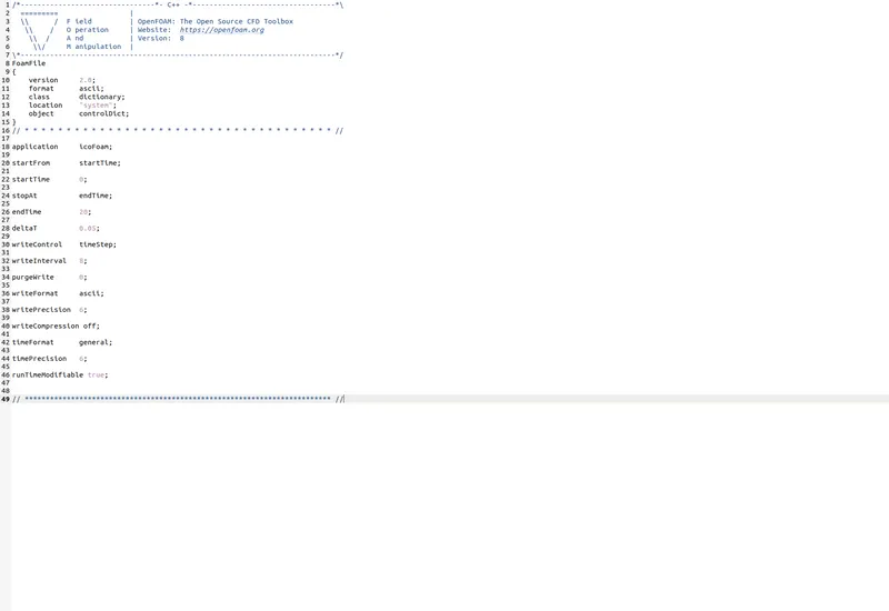
As our maximum velocity is about 0.2 meter per second and time step size is 0.05 s which is about 1/12th of a second, no mesh shall be skipped and as per the CFL criterion, we are below a value of 1 for our courant number.
Along the radial distance, we take about 20 nodes as it is only 1 cm in magnitude. Also, nodes near wall of pipe are finer than at the centre due to boundary thickness and prominent changes in near wall conditions.
A simple grading of 0.2 is taken in y/radial direction.
Boundary Type:
As specified in the problem, the boundary condition to be taken is wedge type. Thus, we shall be considering an angle of theta of less than 5 degrees as can be read from the OpenFoam documentations too.
The below image has been taken from the OpenFoam documentations, the link for which has also been given.
https://www.openfoam.com/documentation/user-guide/4-mesh-generation-and-conversion/4.2-boundaries
Wedge type boundary is considered for an axi-symmetric case when a very small angle is selected for the geometry and we have only 1 cell running along the plane of symmetry.
U file:
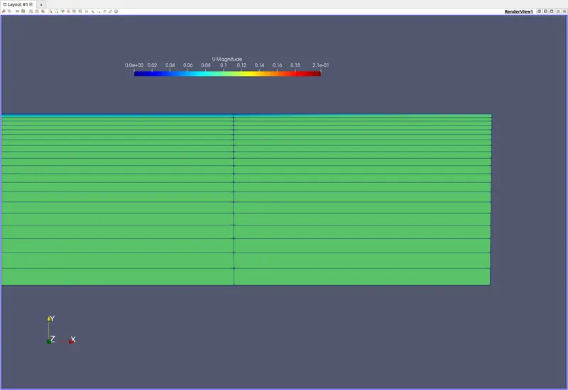
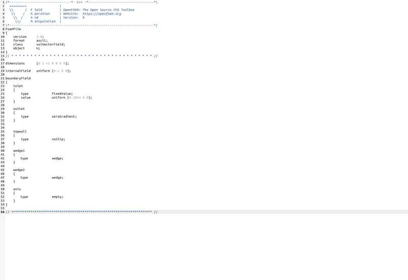
In this dictionary file, for guessed velocity in internal nodes, I have chosen a value of 0.1 as we know the final value shall be around the same. This is also reflected in the outlet geometry meshed image, where the color shown has a magnitude of 0.1. The Image is shown below.
The pressure file:
ControlDict file:
TransportProperties file:
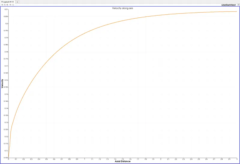
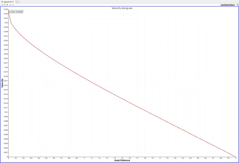
Axial Velocity profile for the length of the pipe
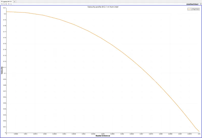
Velocity profile @ 2.1 meters from inlet; This is the fully developed flow region and must be identical to the parabolic nature of velocity profile as shown in literature
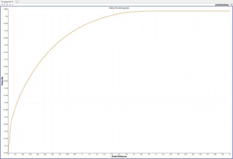
It has been found out that the maximum velocity along the axis, remains constant at about 12 seconds after whoch it has some prominant variations along the axis ( but these variations are still very small in magnitude when compared on a larger scale)
blockMeshDict files - 1 and 2.
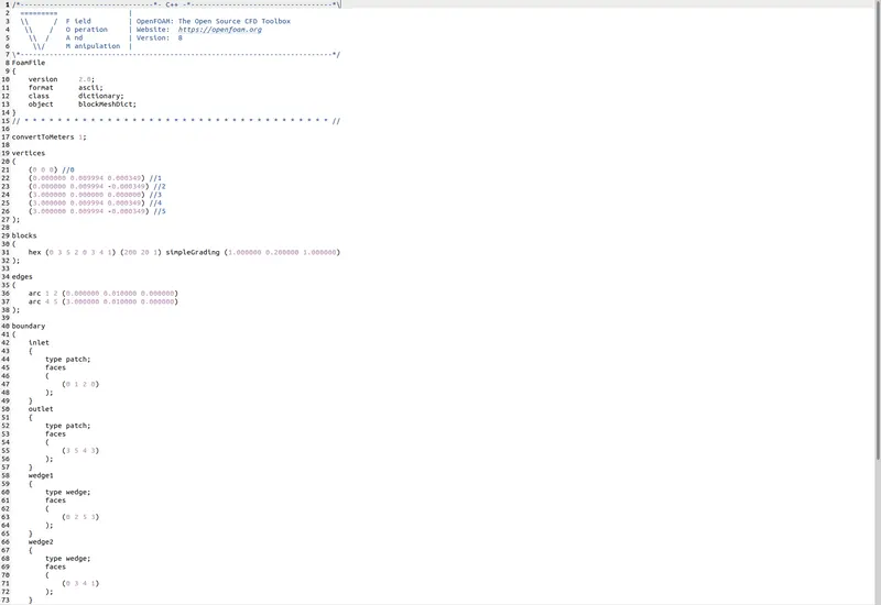
blockMeshDict - 2
Pressure drop along the length of pipe:
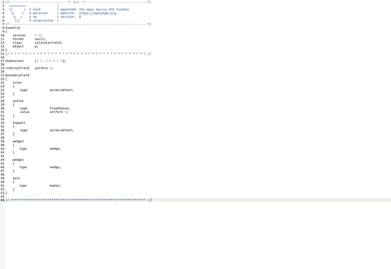
It can be seen from the image that the pressure drop using numerical method is coming to about 32 pascals, which is quiet varied from the analytical value of about 25 pascals.
OpenFoam shows pressure in terms of (m/s)^2, which, as discussed in week 8 challenge, is known as the dynamic or reduced pressure.
Different views of the geometry:
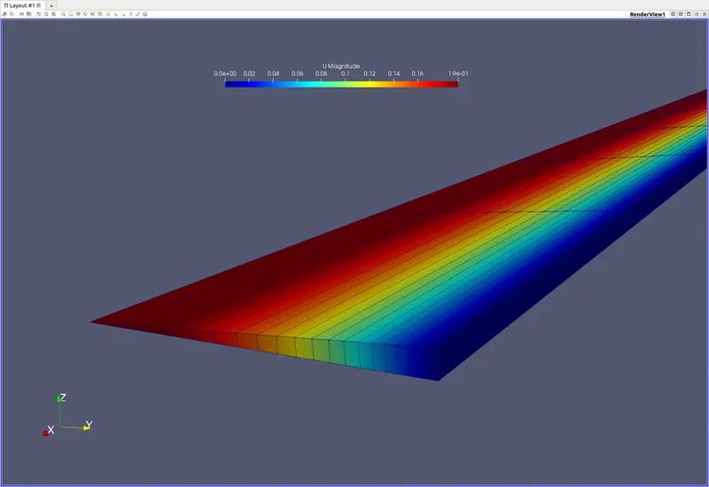
Image - 1
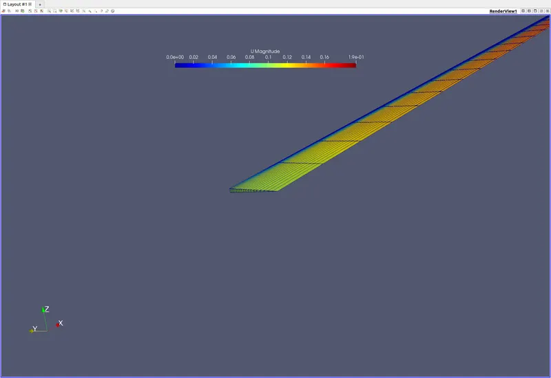
Image - 2
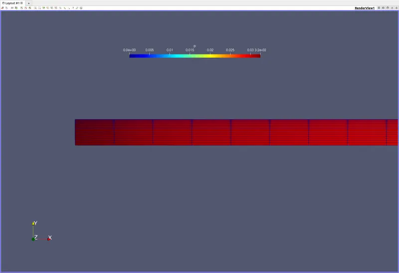
Pressure map
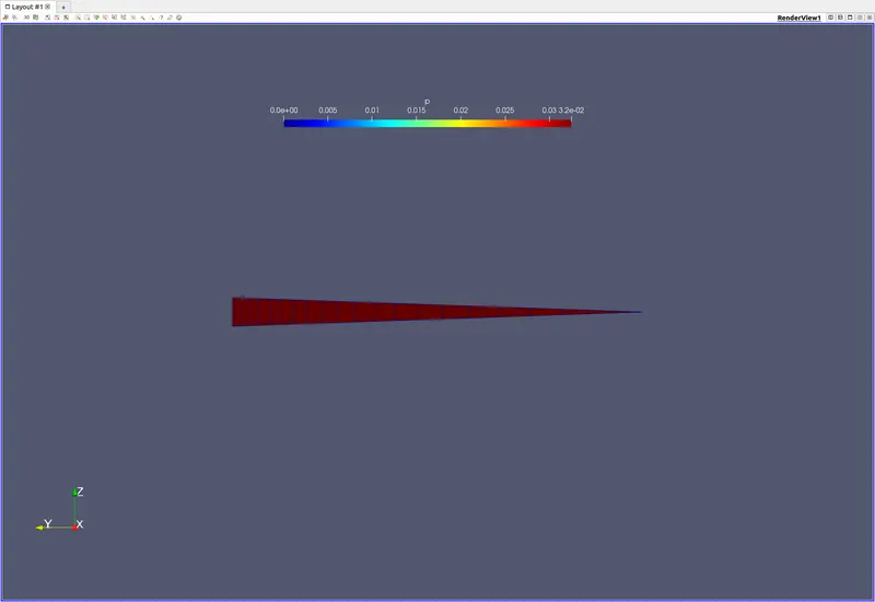
Lateral view of geometry
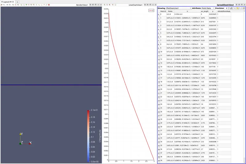
Pressure magnitiude variation along length of geometry
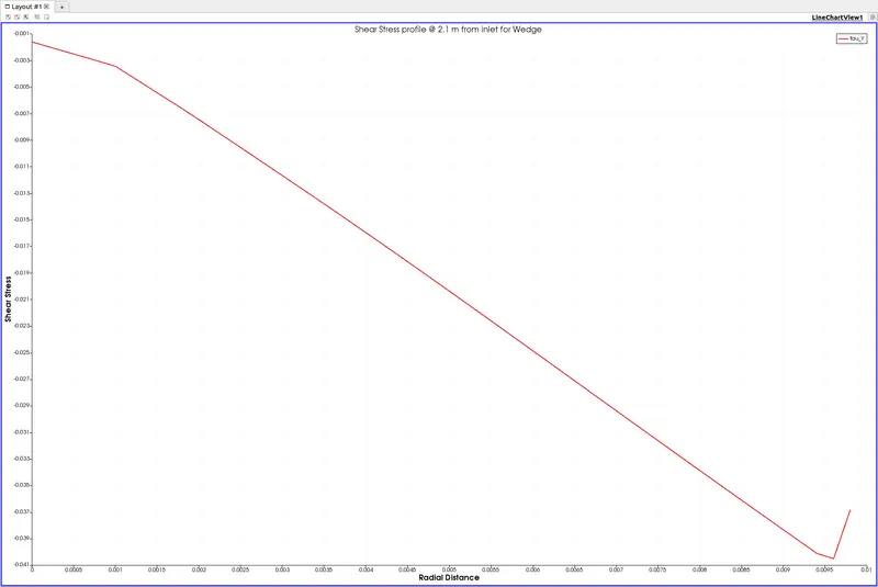
Shear stress profile @ 2.1 meters from Inlet - y magnitude only
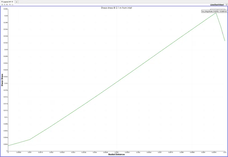
Shear stress profile @ 2.1 meters from Inlet
It must be noted that the shear stress obtained numerically is almost the same as the one obtained analytically using MATLAB script.
- Some errors encountered during execution:
- Once the blockMeshDict file has been generated and copied to the OpenFoam folder, the .txt file extension must be removed by renaming the file. The error else encountered is as shown below.
- Unlike the week 8 challenge, in which the front and back faces of type empty in blockMeshDict file were enconced into a single nested bracket, the same could not be done here. This too, gave an error as shown in images below. Each error image has a description, kindly go through the same.
- Topological error, missing simple terms in blockMeshDict file, in my case, missing semi-colon lead me to this error
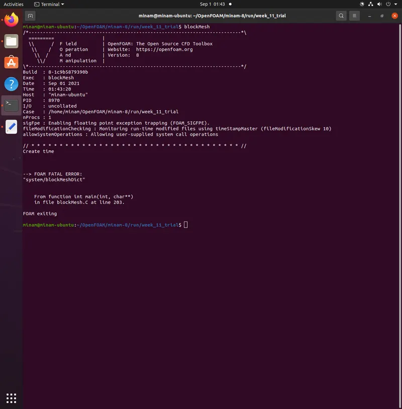
.txt file missing error
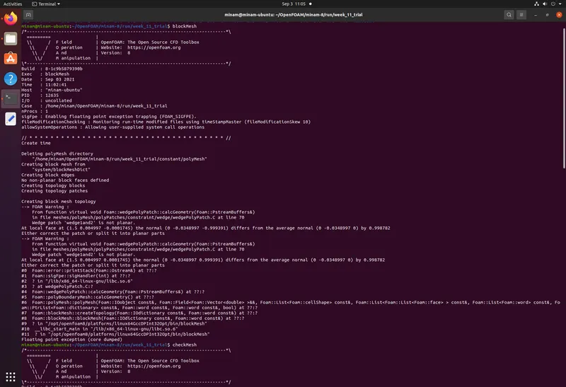
Wedges ensconced into single nested brackets
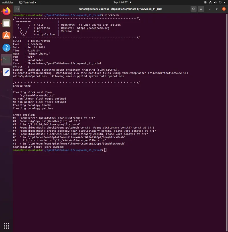
Topological error
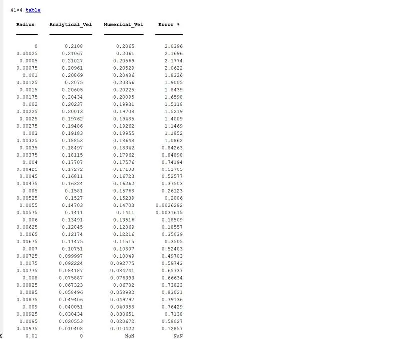
Variation between velocity profile obtained between analytical and numerical results.
Supporting documents for running the MATLAB script successfully have been attached in the report.
Important Points:
- The MATLAB script is programmed to take inputs from the .csv file extracted from OpenFoam for U magnitude at a distance of 2.1 meters from Inlet and also calculates analytical velocity distribution for a fully developed flow. These values and there variational errors and then calculated and tabulated in MATLAB. A snippet of the table is shown below: