Week 10 - Simulating Combustion of Natural Gas.

In this simulation, we have performed a combustion simulation on the combustor model and plotted the variation of the mass fraction of the different species in the simulation using line probes at different locations of the combustor.

Plots for CO2, H2O, CH4, N2, O2, NOx emissions & Soot formation have been attached.

Theory of NOx and soot formations along with the basic species transport have been discussed.

Reactions used in this challenge are shown.

Modelling approach and Solver Settings have been shown.

Results, post processing and conclusions have been discussed.

Part 1:

A simple combustion using methane and air as inlet has been simulated.

Part 2:

Methane-air-2step method has been used and water by mole fraction varying from 5 to 30 % has been added. Effects have been observed and conclusions inferred therein.

Theory:

1. Species Transport:

Ansys Fluent can model the mixing and transport of chemical species by solving conservation equations describing convection, diffusion, and reaction sources for each component species.

• Volumetric Reactions:

Theoretical information about species transport related to volumetric reactions is presented below.

• Species Transport Equations

When we choose to solve conservation equations for chemical species, Ansys Fluent predicts the local mass fraction of each species, Y_i, through the solution of convection-diffusion equation for the i^th species. This conservation equation takes the general form:

`(∂(ρY_i ))/(∂t)+∇.(ρv ⃗Y_i )=-∇.J ⃗_i+R_i+S_i`

Were,

Ri is net rate of production of species I by chemical reaction.

Si is the rate of creation by addition from the dispersed phase plus any user-defined sources.

First term of the equation is the temporal term

Second term of the equation is the convective term

Third term is the diffusion term.

Mass Diffusion in turbulent flows.

• Diffusion at Inlets

For the pressure-based solver in Ansys Fluent, the net transport of species at the inlet consists of both convection and diffusion components. The convection component is fixed by the user-defined inlet species mass fraction. The diffusion component, however, depends on the gradient of the computed species field at the inlet. Thus, the diffusion component (and therefore the net inlet transport) is not specified a priori.

• The Eddy-Dissipation Model:

For mixed-is-burned approximation, Ansys Fluent provides a turbulence-chemistry interaction

model, based on the work of Magnussen and Hjertager, called the eddy-dissipation model. In this model, the chemical reaction rate is governed by the large-eddy mixing time scale, , as in the eddy-breakup model of Spalding. Combustion proceeds whenever turbulence is present ( ), and an ignition source is not required to initiate combustion.

In our present case, we are not concerned with an ignition delay or detailed study of flame start-up. The objective is to ascertain a uniform distribution of temperature at the outlet and to study emissions of NOx and soot at outlet. Since our mixing is turbulent in nature, resulting in a non-zero value of k and epsilon, we shall use the said model for aforementioned reasons.

1. NO_x Model:

The following section presents theoretical background of NO_x prediction.

NO_x emission consists of mostly nitric oxide (NO), and to a lesser degree nitrogen dioxide (NO2) and

nitrous oxide (N₂O). NO_x is a precursor for photochemical smog, contributes to acid rain, and causes

ozone depletion. Thus, NO_x is a pollutant.

The Ansys Fluent NO_x model provides the capability to model thermal, prompt, and fuel NO_x Formation, along with an N₂O intermediate model.

To predict NO_x emissions, Ansys Fluent solves a transport equation for nitric oxide (NO) concentration.

The NO_x transport equations are solved based on a given flow field and combustion solution. In other words, NO_x is postprocessed from a combustion simulation.

In laminar flames and at the molecular level within turbulent flames, the formation of NO_x can be

attributed to four distinct chemical kinetic processes: thermal NO_x formation, prompt NO_x formation, fuel NO_x formation, and intermediate N₂O.

Thermal NO_x is formed by the oxidation of atmospheric nitrogen present in the combustion air.

Prompt NO_x is produced by high-speed reactions at the flame front.

Fuel NO_x is produced by oxidation of nitrogen contained in the fuel.

In Intermediate N₂O model, NO_x may be formed at elevated pressures and oxygen-rich conditions, from molecular nitrogen (N₂) via N₂O.

Since our fuel (methane) does not contain nitrogen and case set-up is not modelled at elevated pressure, we do not need fuel NO_x and intermediate N₂O model.

• Governing Equations for NO_X Transport

Ansys Fluent solves the mass transport equation for the NO species, taking into account convection,

diffusion, production, and consumption of NO and related species. This approach is completely general, being derived from the fundamental principle of mass conservation.

For thermal and prompt NO_x mechanisms, only the NO species transport equation is needed:

`(∂(ρY_(NO) ))/(∂t)+∇.(ρv ⃗Y_(NO) )=∇.(ρD∇Y_(NO))+S_(NO)`

Were,

D is the effective diffusion coefficient.

Y_NO is mass fraction of NO in gas phase.

• Thermal NO_X formation – Extended Zeldovich mechanism

The formation of thermal NO_X is determined by a set of highly temperature-dependent chemical reactions known as the extended Zeldovich mechanism. The principal reactions governing the formation of thermal NO_X from molecular nitrogen are as follows:

`O+N_2 (↔ ) N+NO`

`N+O_2 (↔ ) O+NO`

A third reaction has been shown to contribute to the formation of thermal NO_X, particularly at near stoichiometric conditions and in fuel-rich mixtures:

`N+OH ↔ H+NO`

• Determining O radical Concentration

In order to solve equations from source terms, concentration of O and free radical OH will be required, in addition to the concentration of stable species (that is, N₂, O₂).

Zeldovich suggested considering equilibrium values of temperature, stable species, O atoms, and OH radicals. However, radical concentrations (O atoms in particular) are observed to be more abundant than their equilibrium levels.

To determine the O radical concentration, Ansys Fluent provides the equilibrium, partial equilibrium,

and the predicted concentration approaches.

• Equilibrium Approach

The kinetics of the thermal NOx formation rate is much slower than the main hydrocarbon oxidation

rate, and so most of the thermal NOx is formed after completion of combustion. Therefore,

the thermal NOx formation process can often be decoupled from the main combustion reaction

mechanism and the NOx formation rate can be calculated by assuming equilibration of the

combustion reactions. Using this approach, the calculation of the thermal NOx formation rate is

considerably simplified.

• Partial Equilibrium Approach

An improvement to Equilibrium approach can be made by accounting for third body reactions in O2 dissociation-recombination process.

Thus, we shall consider the standard Equilibrium approach.

• Determining OH Radical Concentration

One of the approaches is an exclusion of OH concentrations, by assuming third reaction of the extended Zeldovich mechanism to be negligible. This assumption holds good and is justified for lean fuel conditions.

Thus, we shall exclude OH concentration in our case setup.

• Prompt NO_X Formation

Prompt NO_X is most prevalent in rich flames. The actual formation involves a complex series of reactions and many possible intermediate species.

A number of species resulting from fuel fragmentation have been suggested as the source of prompt

NO_X in hydrocarbon flames (for example, CH, CH₂, C, C₂H), but the major contribution is from CH and CH₂.

The products of these reactions could lead to formation of amines and cyano compounds that

subsequently react to form NO.

Prompt NO_X formation is proportional to the number of carbon atoms present per unit volume and

is independent of the parent hydrocarbon identity.

2. Soot Model

Ansys Fluent predicts soot concentrations in a combustion system using one of the following

available models:

• The One-step Khan and Greeves model
• The Two-step Tesner model
• The Moss-Brookes model
• The Moss-Brookes-Hall model
• The Method of Moments model

The Moss-Brookes model, in which Ansys Fluent predicts soot formation for methane flames (and higher hydrocarbon species, if appropriately modified) by solving transport equations for normalized radical nuclei concentration and the soot mass fraction. This model has less empiricism and should theoretically provide better accuracy than the Khan and Greeves and Tesner models.

The Moss-Brookes model solves transport equations of normalized radical nuclei concentration and soot mass fraction.

`(∂(ρY_(so ot)) )/(∂t)+∇.(ρv ⃗Y_(so ot) )=∇.( μ_t/σ_(so ot) ∇Y_(so ot) )+(dM)/dt`

`(∂(ρb_(n uc)^** ))/(∂t)+∇.(ρv ⃗b_(n uc)^** )=∇.(μ_t/σ_(n uc) ∇b_(n uc)^**)+1/N_(norm) (dN)/dt`

Were,

`Y_(so ot)` = soot mass fraction

M = soot mass concentration (kg/m³)

`b_(n uc)^**` = normalized radical nuclei concentration (particlesx10^-15 /kg) = `N/(ρN_(no rm) )`

N = soot particle number density (particles/m³)

`N_(norm)` = 10¹⁵ particles

Fenimore-Jones Model:

This model takes into account the soot oxidation due to the hydroxyl radical.

1. Reactions – Methane-air

The mechanism of this reaction has one principal reaction as shown below

`CH_4+2(O_2+3.76N_2 )=CO_2+2H_2 O+7.52N_2`

Mole Fraction of Air:

• Oxygen – 2/9.52 = 0.21
• Nitrogen – 7.52/9.52 = 0.79

Mass Fraction of Air:

• Oxygen – 64/274.56 = 0.23
• Nitrogen – 210.56/274.56 = 0.77

1. Reactions – Methane-air-2step

The mechanism of this reaction has two principal reactions as shown below

`CH_4+3/2 (O_2+3.76N_2 )=CO+2H_2 O+5.64N_2`

`CO+1/2 O_2 = CO_2`

Mole and mass fraction is same as above.

In Ansys Fluent, when modelling combustion of a methane-air mixture using global kinetics, we do not need to explicitly specify the species involved in the reaction or the reaction itself. Simply selecting methane-air or methane-air-2step for case 1 and case 2 respectively as the mixture material to be used, and the relevant species (that is, CH4, O2, CO2, H2O, N2) and reaction data will be loaded into the solver from the database.

Species, reactions and other properties can be checked and/or modified from Create-Edit Materials dialog box.

Geometry:

• Open SpaceClaim and import the geometry.
• Under Design tab, select plane and choose the XY plane.
• Now, select Split Body command under Design tab and select the body to be cut, followed by selecting the XY plane.
• After the body is split, click on the side we need to remove.
• Repeat the process for the inner 2 bodies as well.
• Since we won’t be modelling an actual burner with flame or rather, flame modelling is not being done, we can combine all the internal bodies into one thereby using Eddy Dissipation model which instigates combustion based on k and epsilon values from turbulence models.
• Repeat the process for XZ plane and remove the lower half of the remainder.
• A quadrant of a burner remains, click in Z axis to get normal view of XY plane.
• Using Combine command under Design tab, join the three bodies.
• Click on the faces and copy these to a new file.
• Save and close SpaceClaim
• Right click on geometry and load the modified geometry into SpaceClaim.
• Go to meshing.

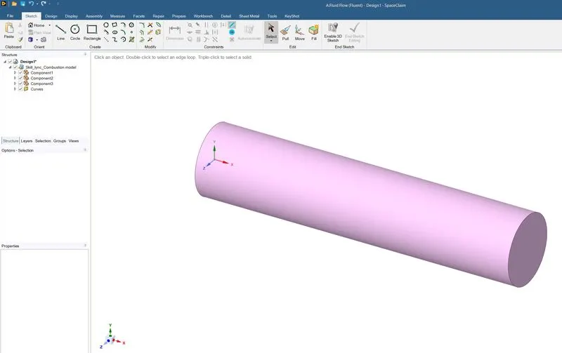
3D Model

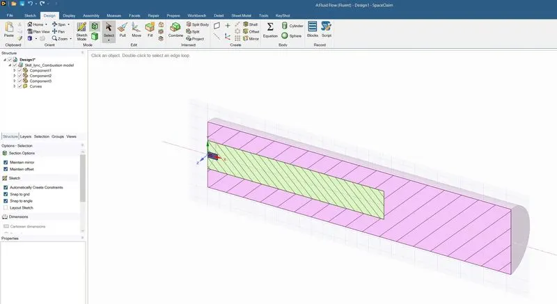
Cut View

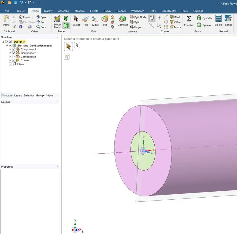
Creating XY Plane

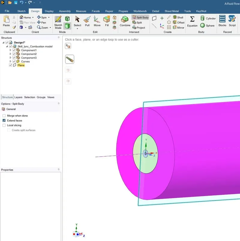
Creating XY Plane 2

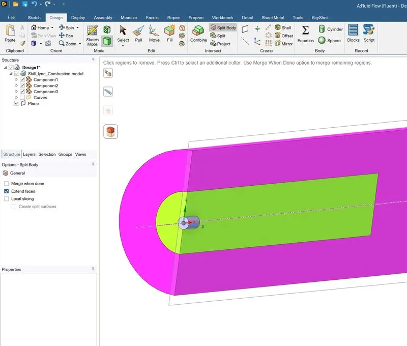
Creating XY Plane 3

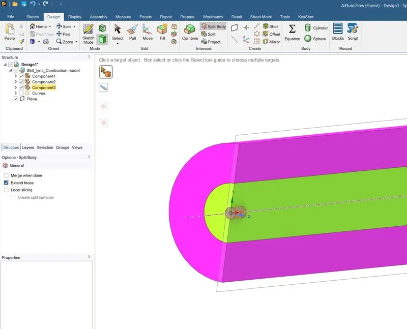
Creating XY Plane 4

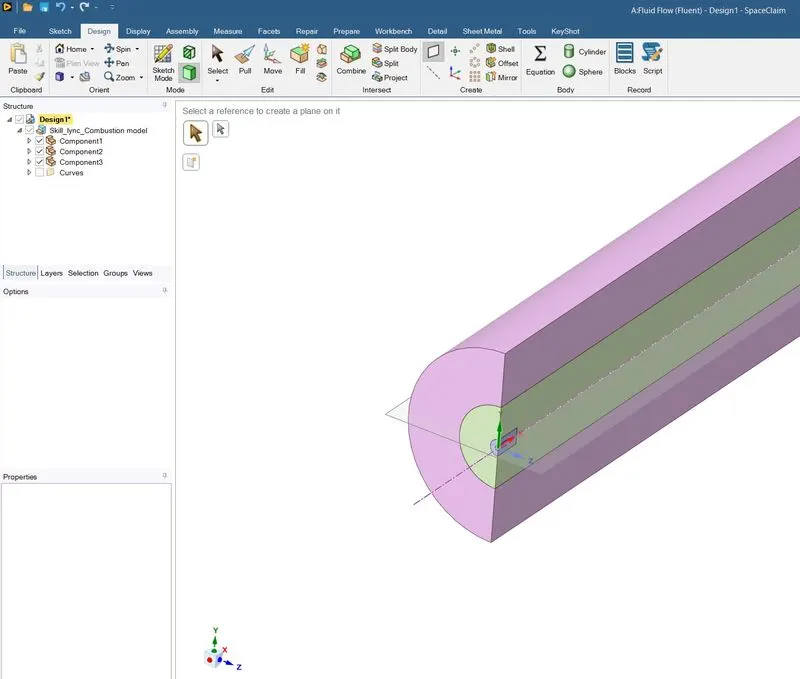
create XZ plane

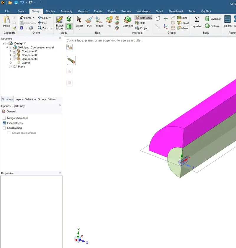
create XZ plane 2

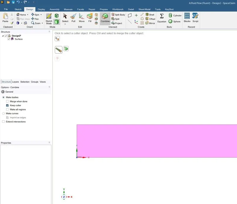
combine bodies

Meshing:

• Since the geometry is very simple, we can either use cartesian or all triangles meshing. All triangles Method has been used for this simulation.
• Element quality check shows decent quality for a size of 1 mm.
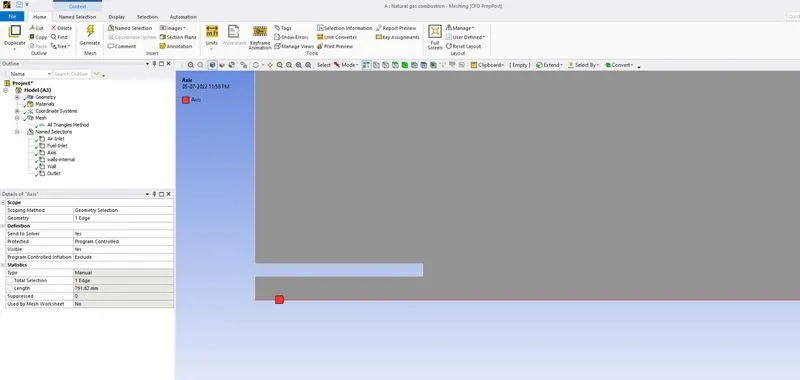
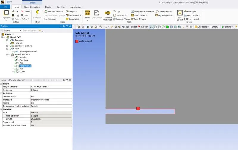
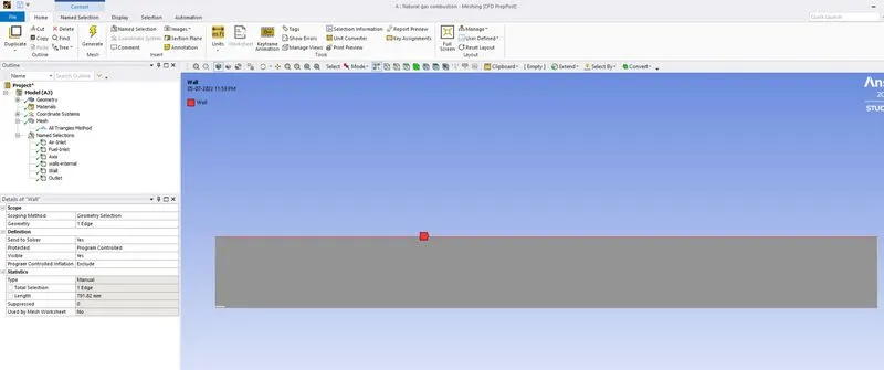
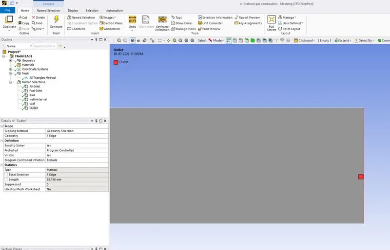
• Named Selection as Air and Fuel Inlet, Axis, Outlet and walls have been shown in images below.
• It is to be noted that axis type needs to be modified in Fluent to symmetry or walls, or change the setup to an axisymmetric simulation. We have done the later.

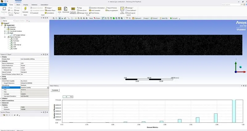
Mesh Quality

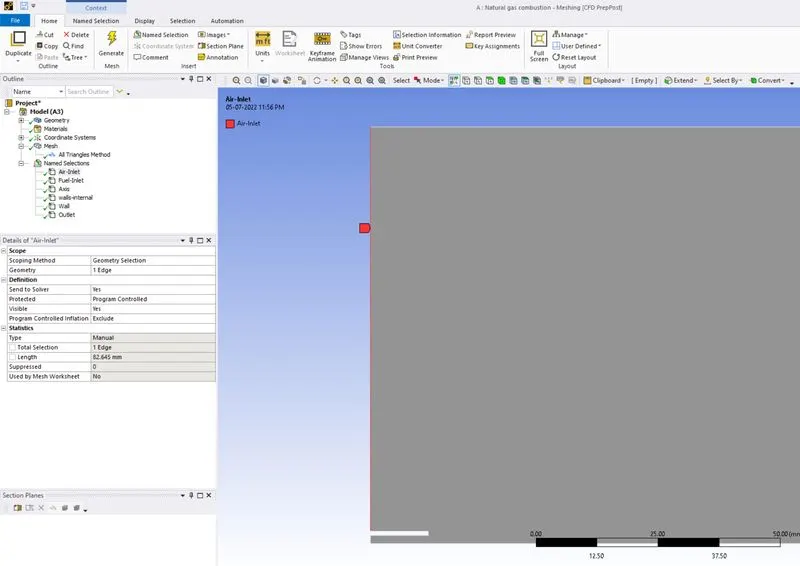
Air-Inlet

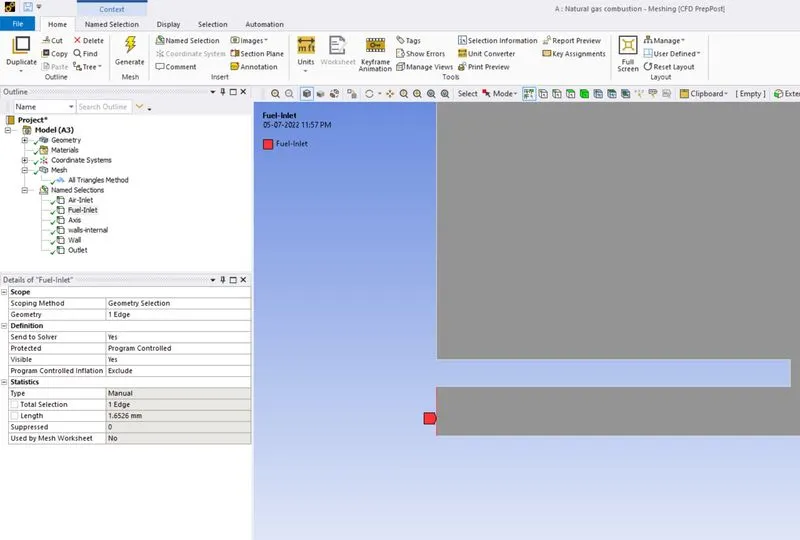
Fuel-Inlet

Axis

Walls-Internal

Wall

Outlet

Steps in Fluent:

1. Generic Steps

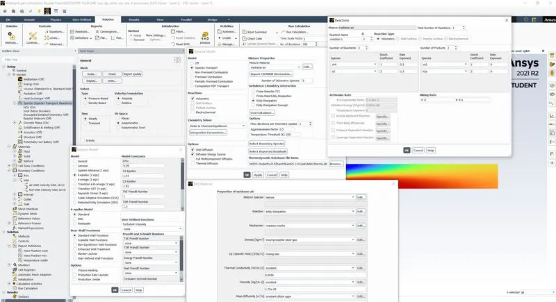
Under Setup, General and Models choose the following:

• Pressure-Based Solver
• Axisymmetric 2D space
• Absolute Velocity Formulation.
• Under Model, turn on energy mode.
• Under Viscous Model, choose k-epsilon model with standard k-epsilon model specification and Near-Wall treatment is set to Standard wall function.
• K-epsilon model is selected as Eddy-Dissipation Model under TCI shall be chosen. Theory regarding the same has been discussed above.

Solution Methods

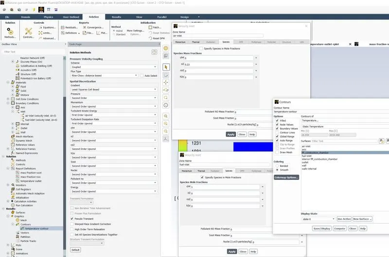
• Pressure-Velocity Coupling Scheme is set to “Coupled” as this is a Steady-State simulation.
• Hybrid Initialization is used as we have multiple Inlets.

2. Overview of User Inputs for Modeling Species Transport

The basic steps for setting up a problem involving species transport and reactions are listed below.

• Under Model, select Species Transport.
• Under Reactions, select Volumetric.
• Under Chemistry Solver, select Relax to Chemical Equilibrium.
• Under Options, check on Inlet Diffusion.
• In the Mixture Material drop-down list under Mixture Properties, select methane-air.
• The number of species in the selected mixture material is displayed in the Number of Volumetric Species field. Since we do not have any solid phase component, Number of Solid Species and Number of Site Species is disabled.
• To review the mixture composition and reactions of the selected Fluent database mixture material, click the View… button to the right of Mixture Material. This opens the Fluent Database Materials dialog box.
• Clicking, in turn, the .. buttons next to Mixture Species and Reaction opens the corresponding dialog boxes allowing us to examine the constituent species and reactions data.
• On clicking either OK or Apply, Ansys Fluent copies Fluent database mixture material including all constituent materials (species) and properties to our current case setup and appears under Mixture in the tree and the Materials task page.
• When the mixture material is copied, the Mixture Material drop-down list in the Species Model dialog box changes to contain only the mixtures defined by us in case setup.
• The .. button is replaced by the Edit... button giving an option to access the Edit Material dialog box from the Species Model dialog box.
• Under Turbulence-Chemistry Interaction (TCI) modeling option, select Eddy-Dissipation.

3. Using/Understanding the Reactions Dialog Box

• Open Species Model dialog box from Species under Setup.
• Select Edit… to the right of Mixture Material under Mixture
• Select Edit… to the right of Eddy Dissipation under Reaction from Edit Material dialog box.
• Total number of Reactions field is set to 1, this is volumetric reactions.
• Number of Reactants and the Number of Products is set to 2, since the species in reactants are CH₄ and O₂ and species in products are CO₂ and H₂
• In a Global forward reaction, there is no reverse reaction, here the product species generally do not affect the forward rate, so the rate exponent for all products is 0.
• For reactant species, rate exponent is not equal to the stoichiometric coefficient when reaction is not an elementary reaction.
• An elementary reaction is reaction between intermediate species formed between Reactants and Products.

4. Using the NO_X and Soot Model

• Set appropriate parameters, as described here…
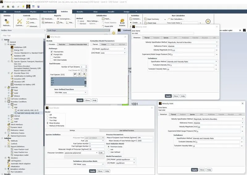
• Setup Þ Models Þ Species Þ NO_X Þ Edit…
• Enable thermal and prompt NO_X
• Define fuel streams for prompt NO_X
• Under Soot Model, select Moss-Brookes Model for soot calculations.
• Soot Oxidation Model is selected as Fenimore-Jones Model

5. Boundary conditions

• Go to Setup Þ Boundary Conditions Þ Inlet Þ air-inlet (user-defined)
• Under Momentum tab, set velocity magnitude to 0.5 m/s
• Under Thermal tab, temperature is specified as 300 K.
• Under species tab, set Species Mass Fraction for oxygen to 0.23
• Go to Setup Þ Boundary Conditions Þ Inlet Þ fuel-inlet (user-defined)
• Under Momentum tab, set velocity magnitude to 80 m/s
• Under Thermal tab, temperature is specified as 300 K.
• Under species tab, set Species Mole Fraction for methane to 1.

CASE 1 - SETUP

General

nox and soot model

species at inlet and methods

Scaled Residuals

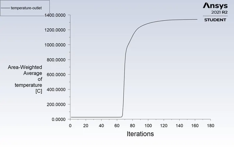
Temperature - outlet

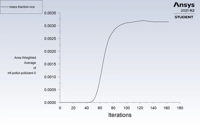
mass fraction nox

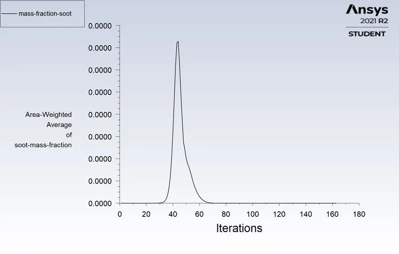
mass fraction soot

CFD POST-PROCESSING

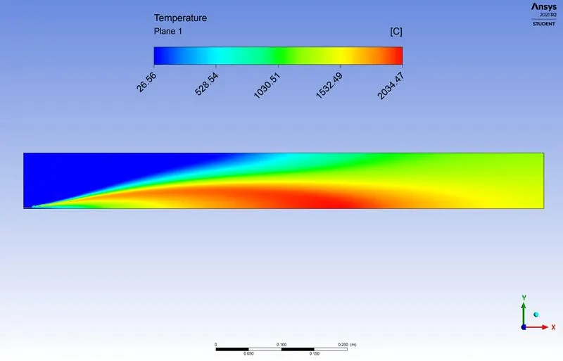
Temperature contour

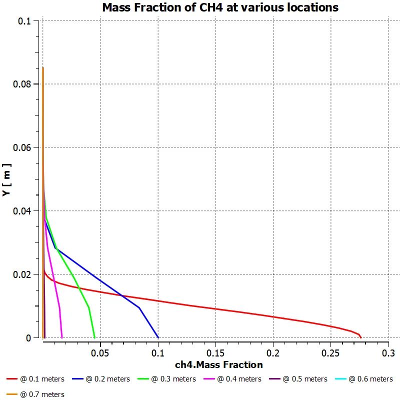
Chart mass fraction methane

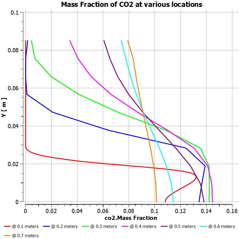
Chart mass fraction CO2

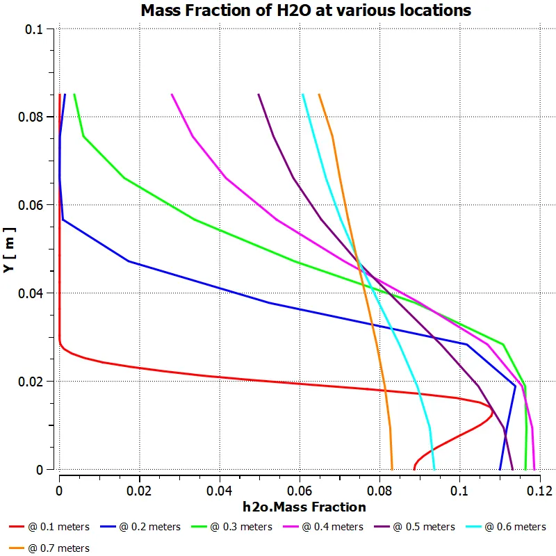
Chart mass fraction H2O

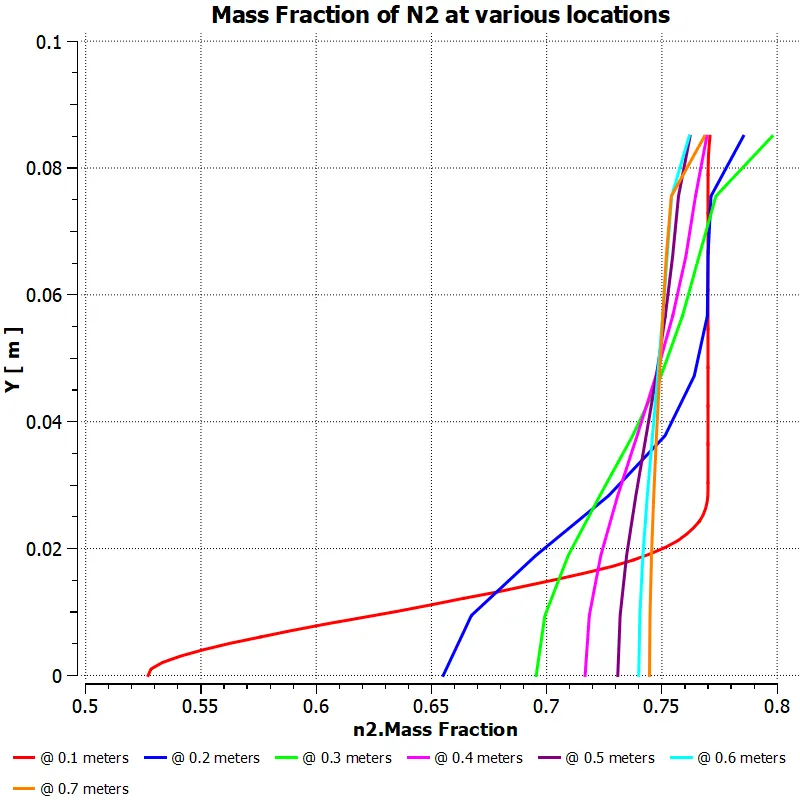
Chart mass fraction N2

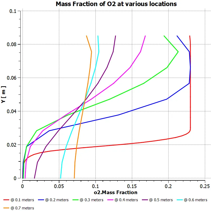
Chart mass fraction oxygen

CASE 2 - METHANE-AIR-2STEP (MOLE FRACTION OF H2O FROM 5-30%)

SETUP

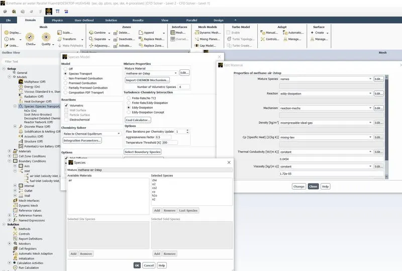
properties of methane-air-2step

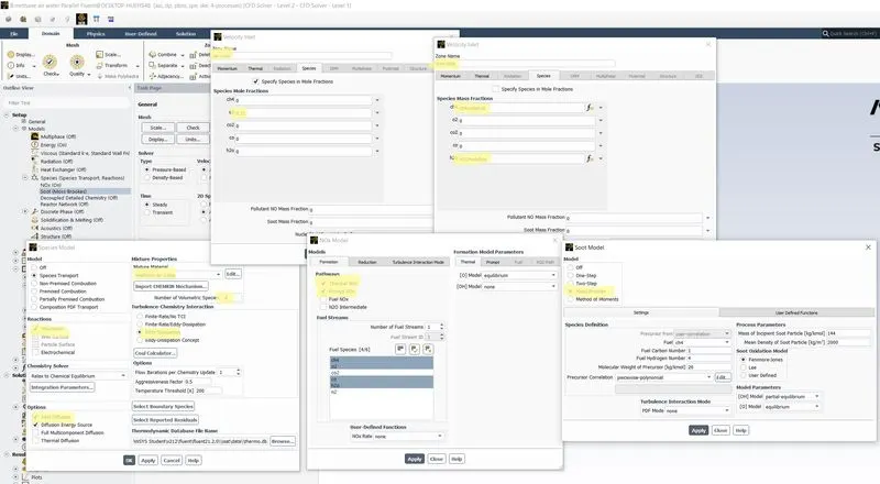
soot and nox models

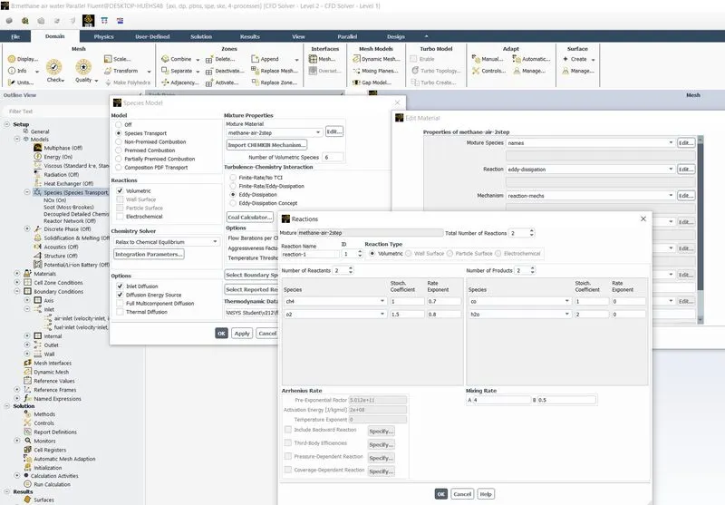
The reactions dialog box

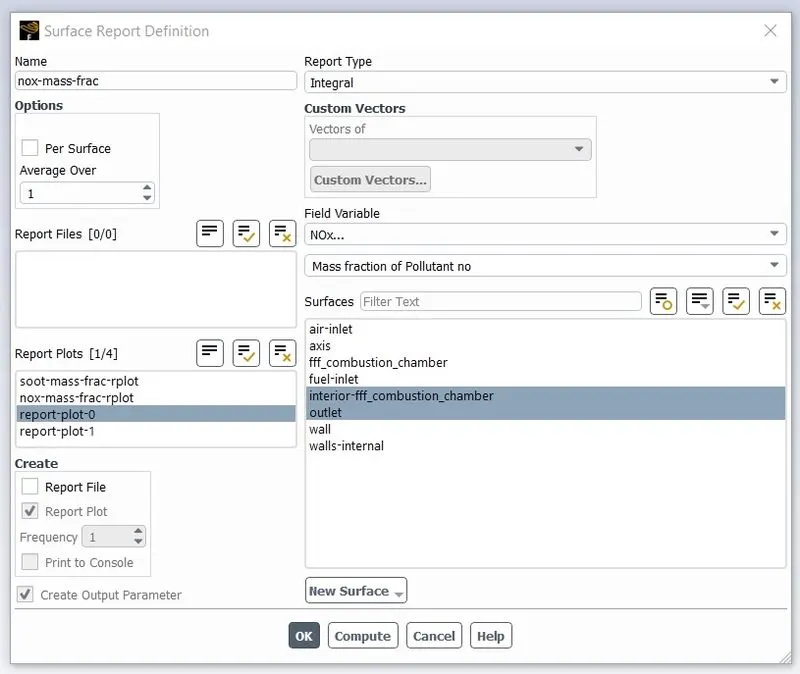
nox surface report and parameter

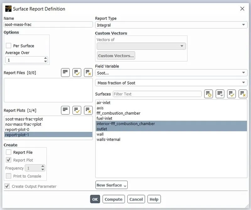
soot surface report and parameter

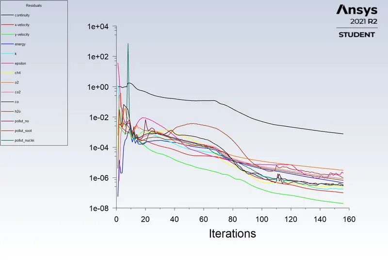
Scaled Residuals

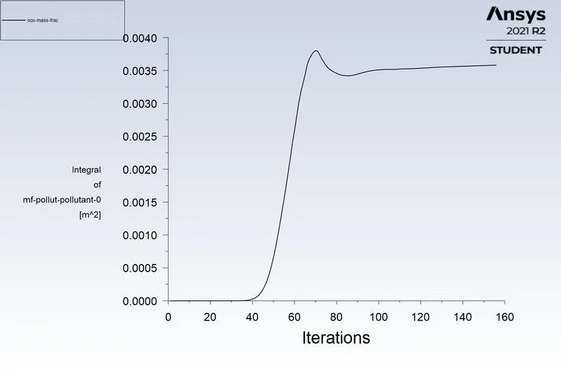
nox mass fraction

soot mass fraction

CFD POST PROCESSING

• 5% mole fraction oxygen

Mass fraction CH4

Mass fraction CO2

Mass fraction CO

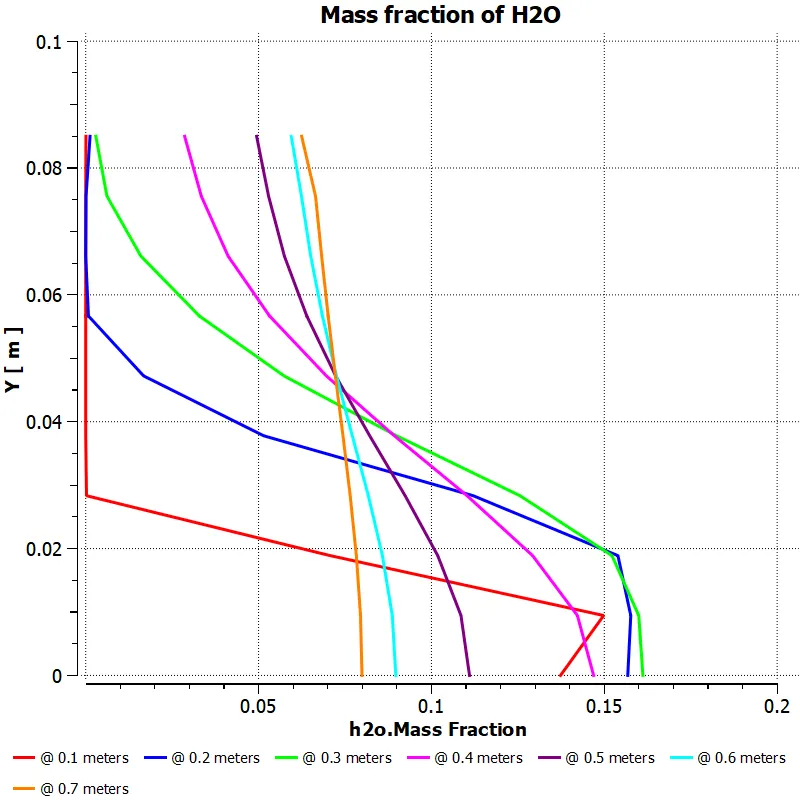
Mass fraction H2O

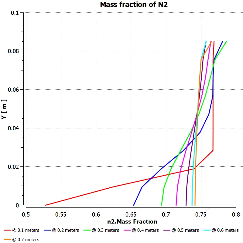
Mass fraction N2

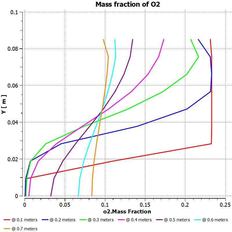
Mass fraction O2

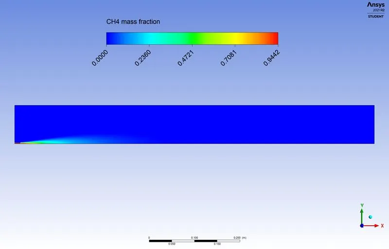
CH4 mass fraction

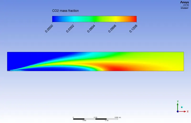
CO2 mass fraction

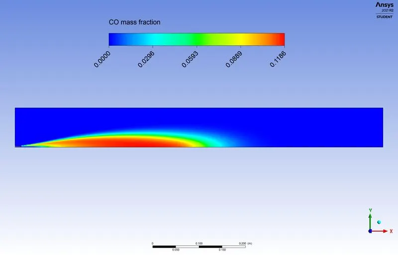
CO mass fraction

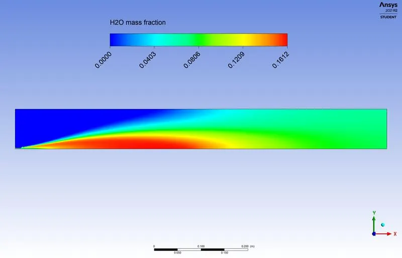
H2O mass fraction

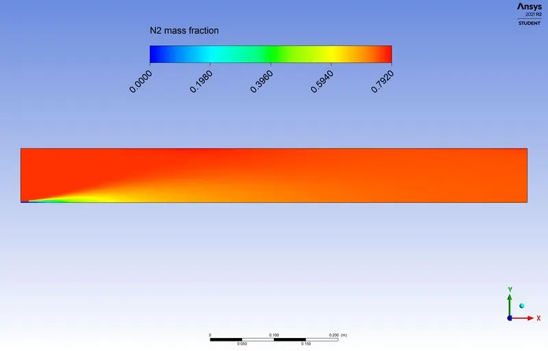
N2 mass fraction

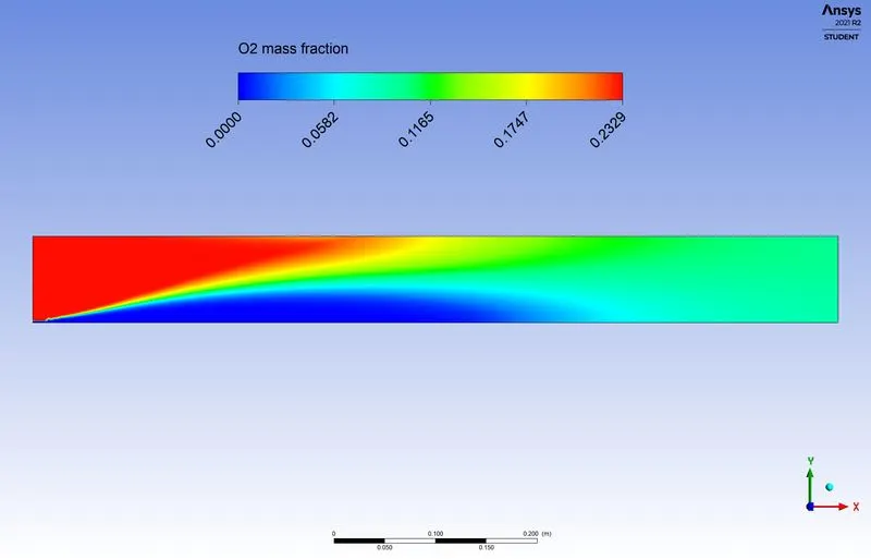
O2 mass fraction

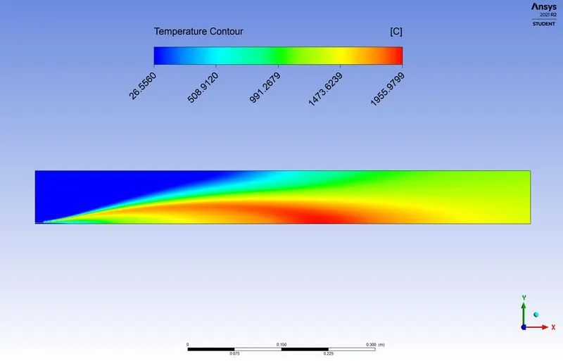
Temperature contour

• 10% mole fraction oxygen

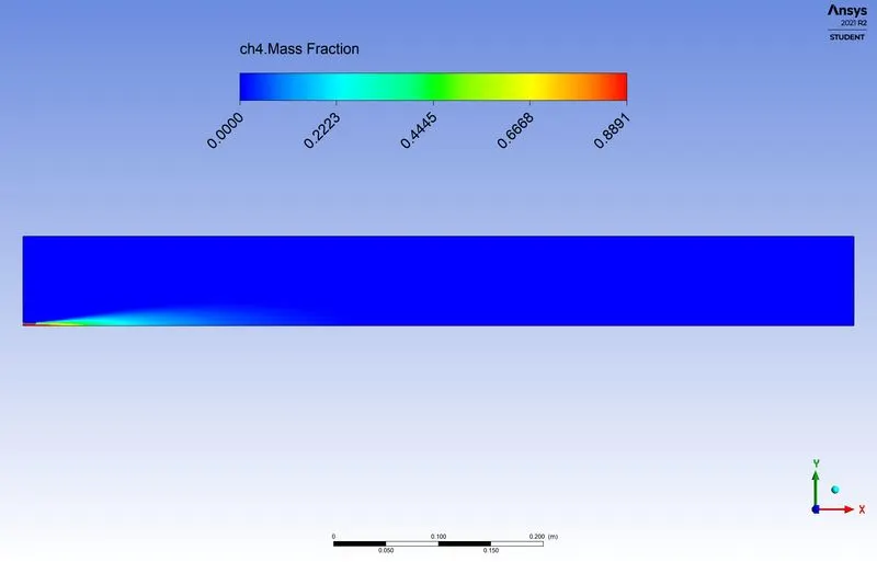
CH4 mass fraction

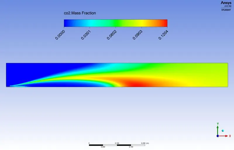
CO2 mass fraction

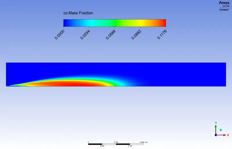
CO mass fraction

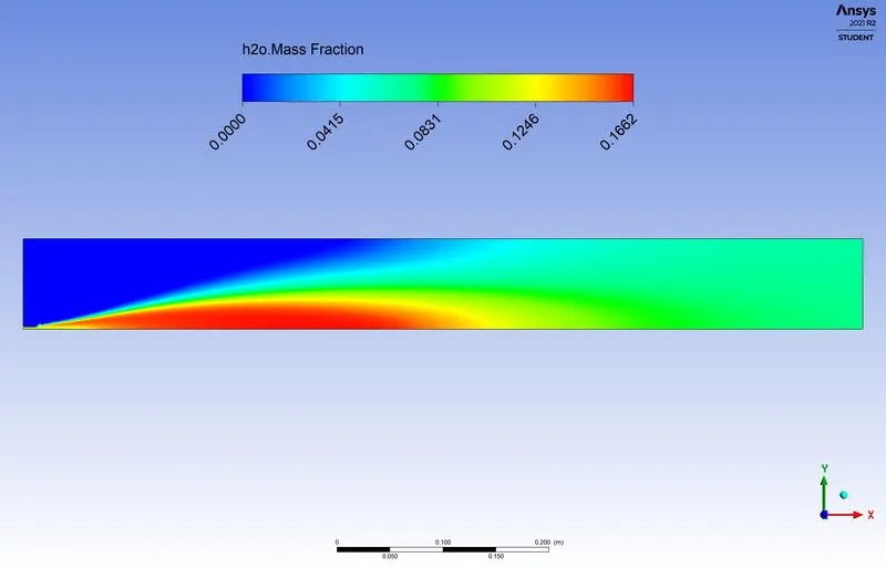
H2O mass fraction

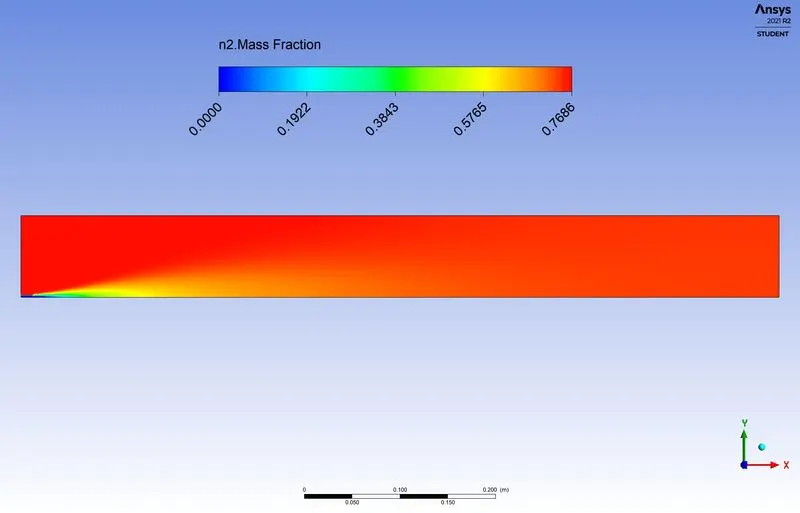
N2 mass fraction

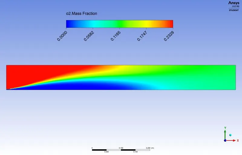
O2 mass fraction

Temperature contour

• 15% mole fraction oxygen

CH4 mass fraction

CO mass fraction

CO2 mass fraction

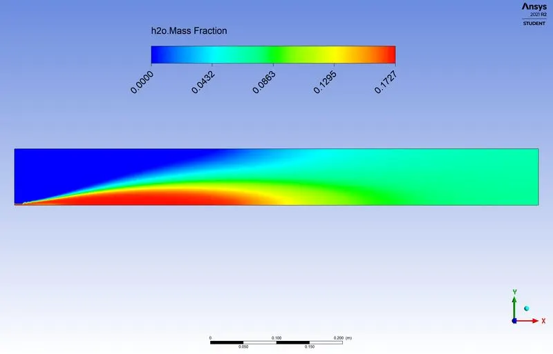
H2O mass fraction

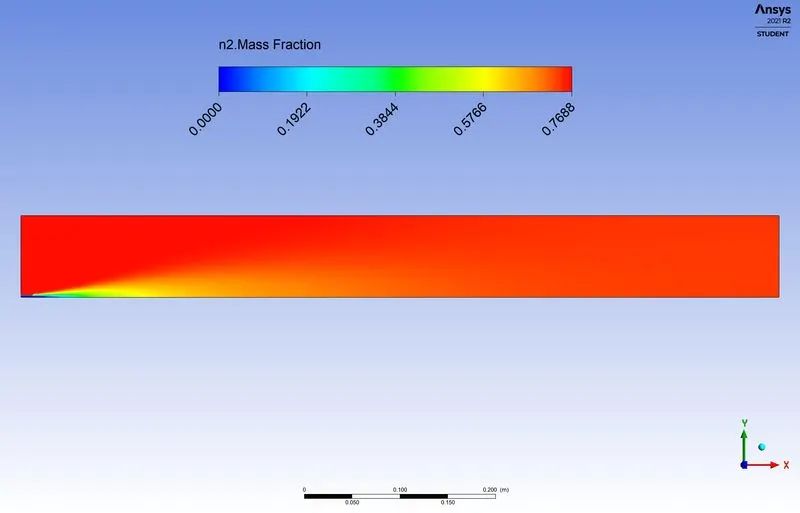
N2 mass fraction

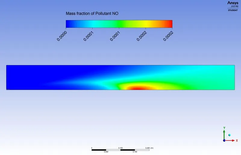
NOx mass fraction

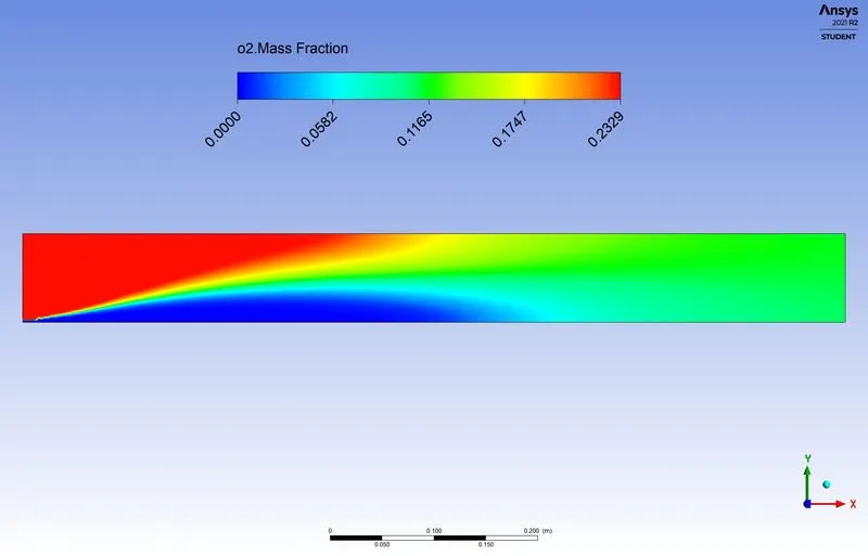
O2 mass fraction

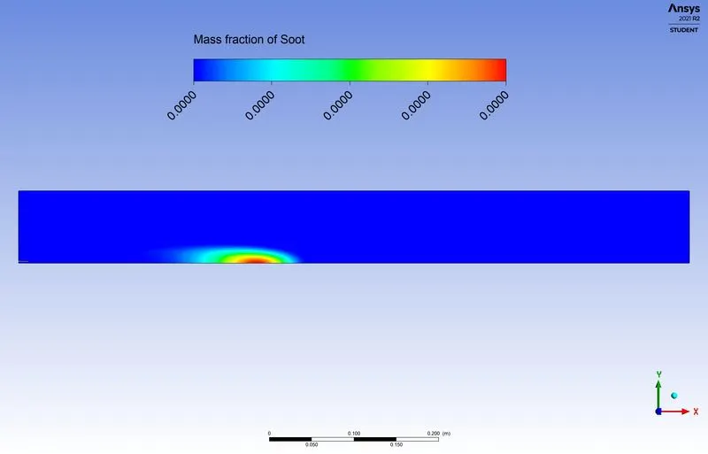
soot mass fraction

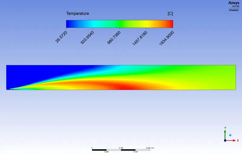
Temperature contour

• 20% mole fraction oxygen

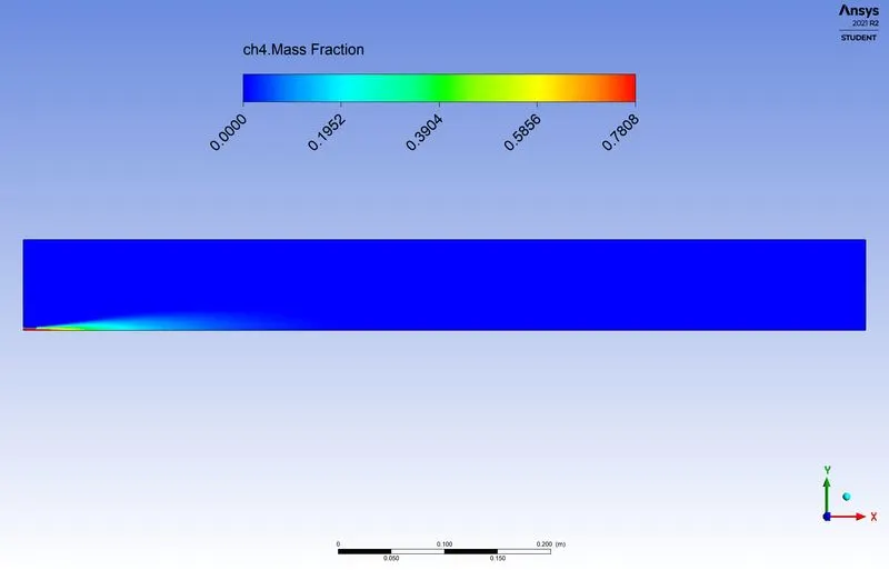
CH4 mass fraction

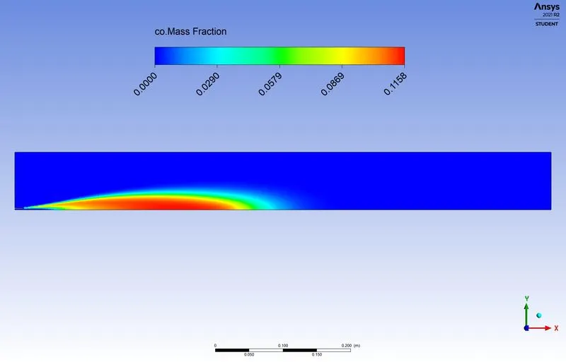
CO mass fraction

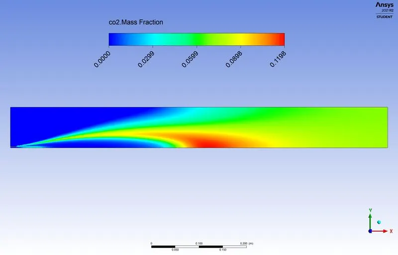
CO2 mass fraction

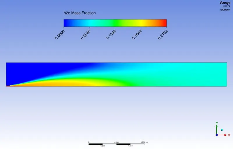
H2O mass fraction

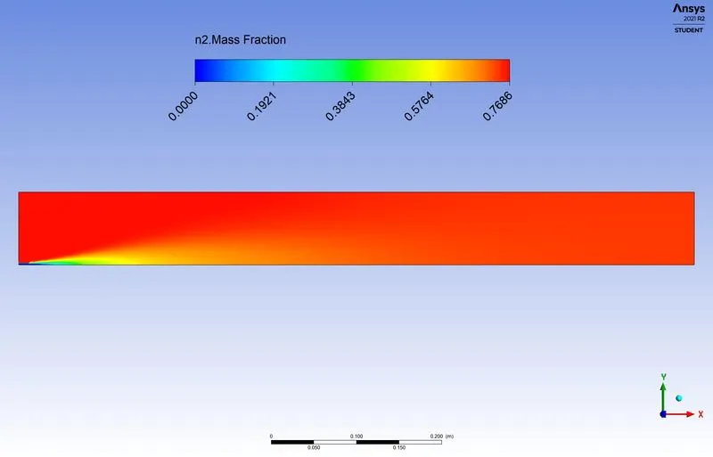
N2 mass fraction

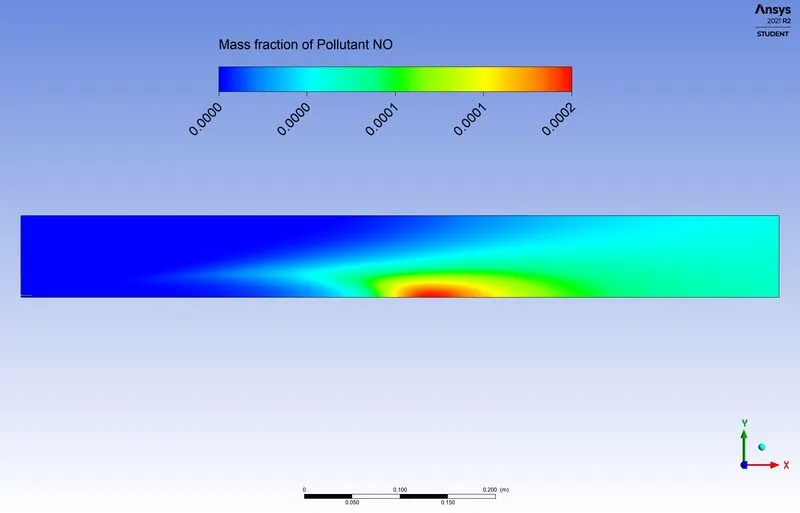
NOx mass fraction

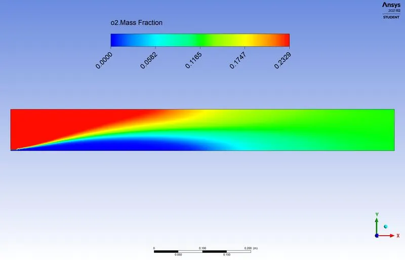
O2 mass fraction

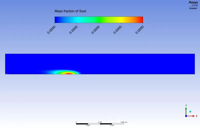
soot mass fraction

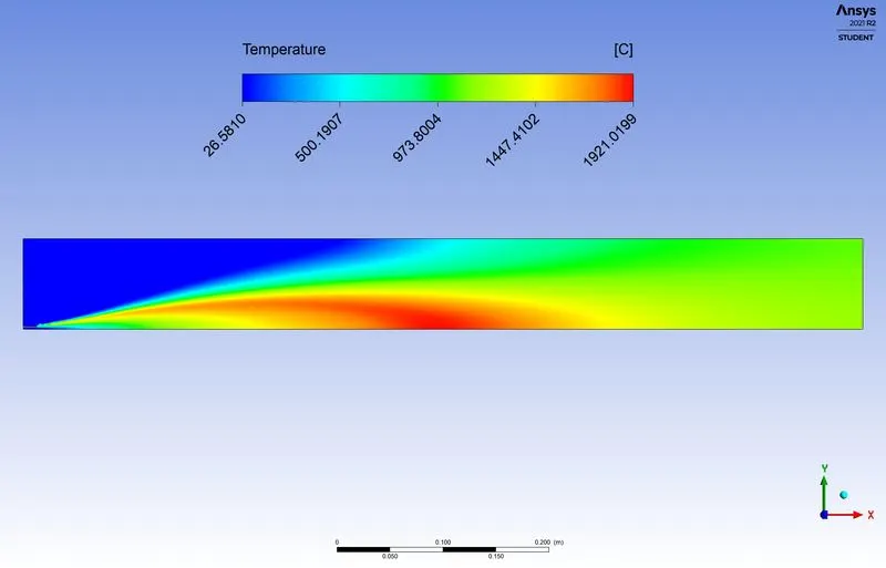
Temperature contour

• 25% mole fraction oxygen

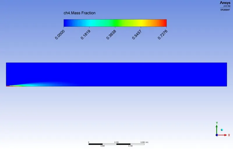
CH4 mass fraction

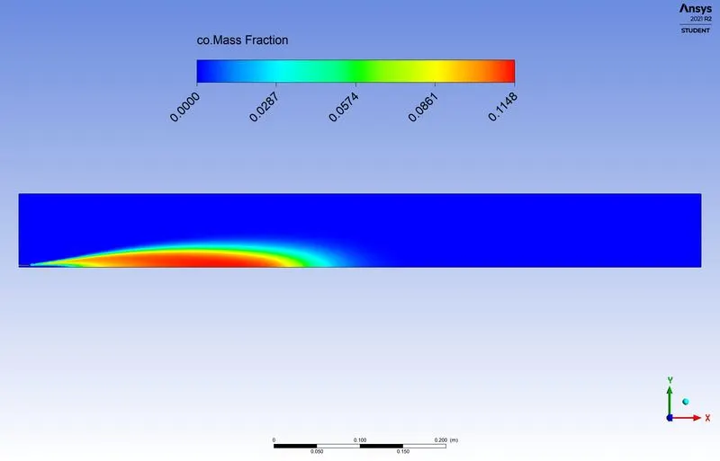
CO mass fraction

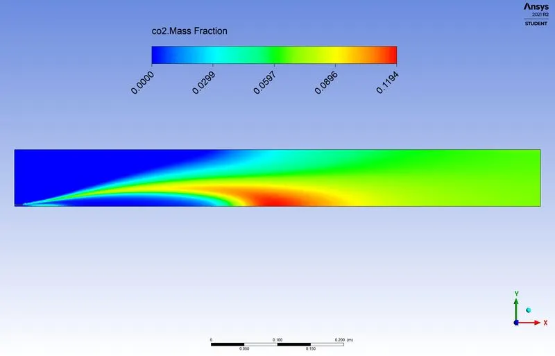
CO2 mass fraction

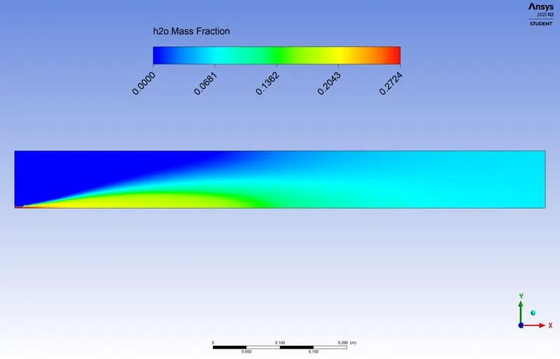
H2O mass fraction

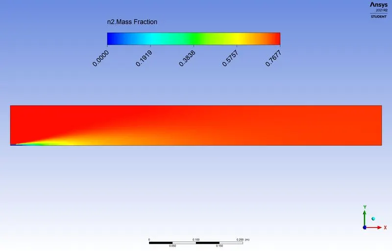
N2 mass fraction

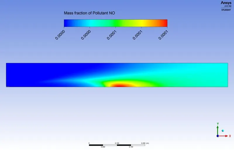
NOx mass fraction

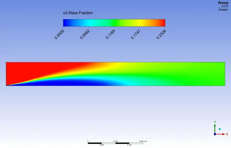
O2 mass fraction

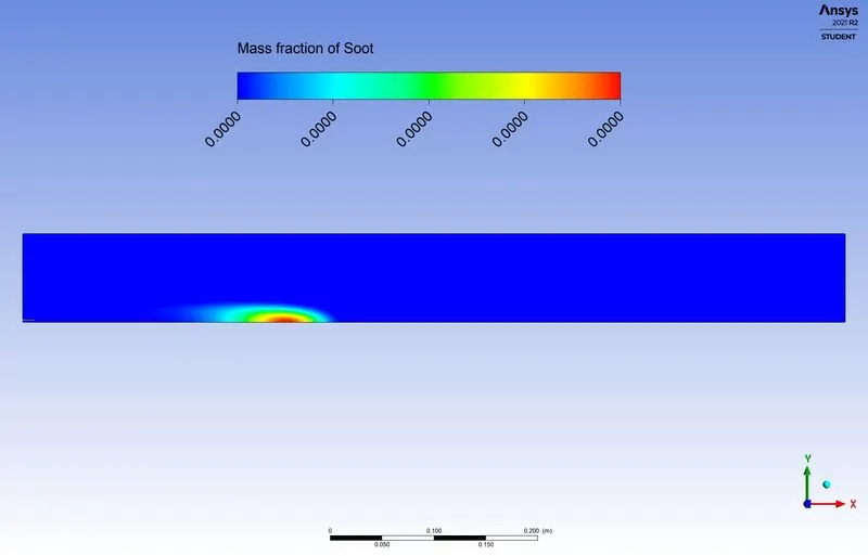
soot mass fraction

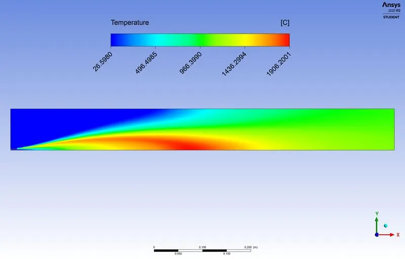
Temperature contour

• 30% mole fraction oxygen

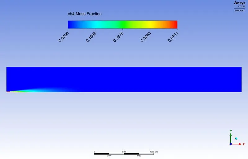
CH4 mass fraction

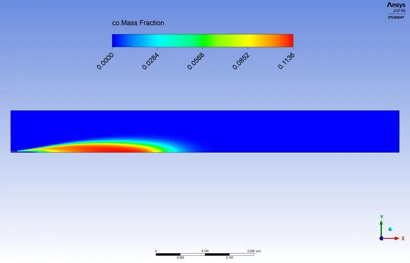
CO mass fraction

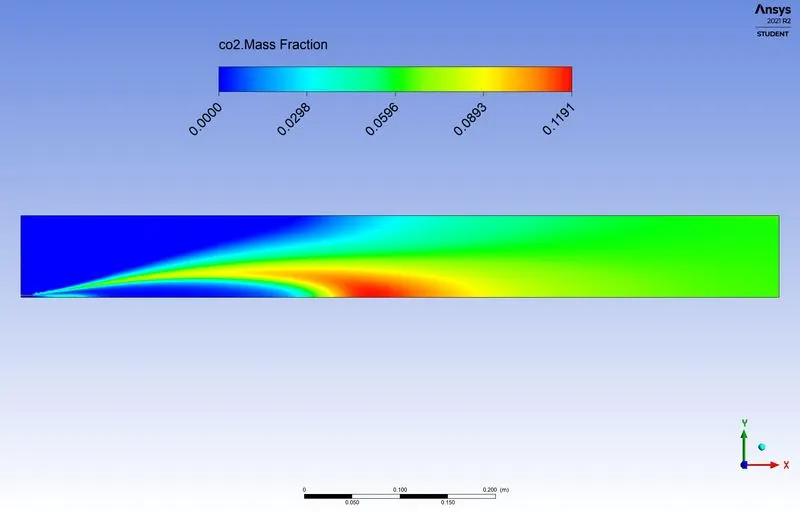
CO2 mass fraction

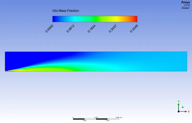
H2O mass fraction

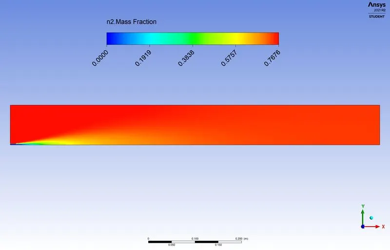
N2 mass fraction

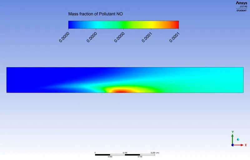
NOx mass fraction

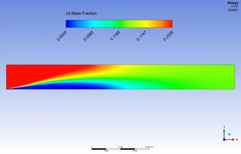
O2 mass fraction

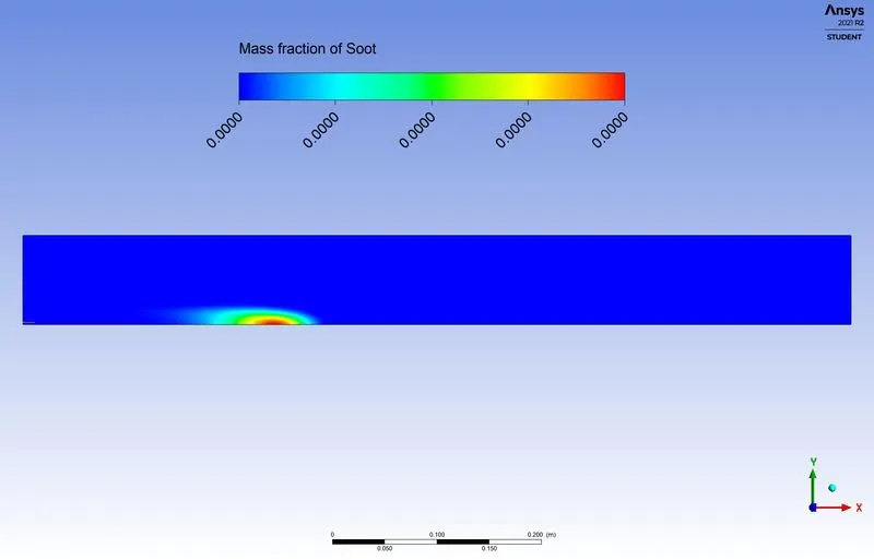
soot mass fraction

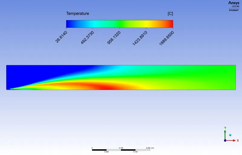
Temperature contour

Post Processing and Parametrization

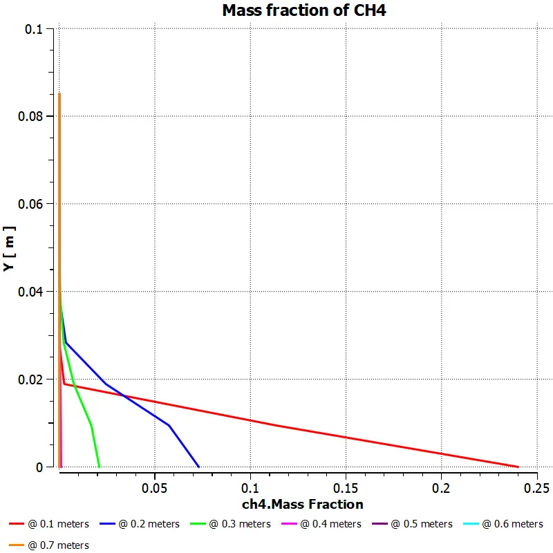
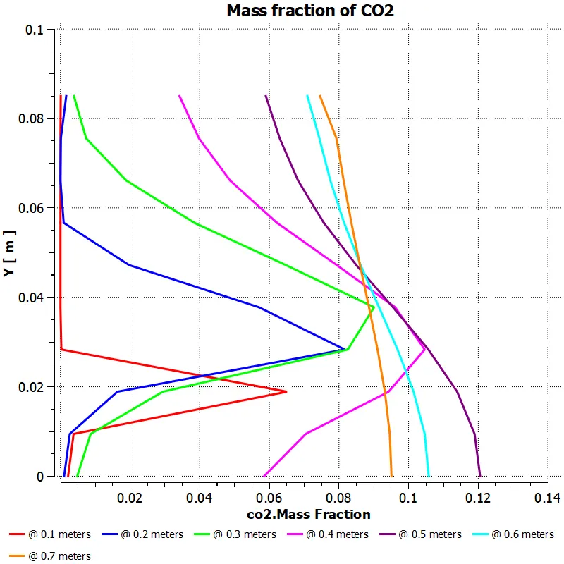
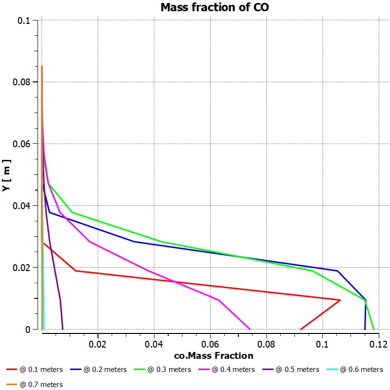
• Line probes for various species from within the domains are used to create line charts which show the variation of these species along the radial direction.
• Contours of species, soot and NOx pollutant have been sown for each case as well.
• Temperature Contours have also been shown for each case.
• Mole fraction of methane and water have been parametrized as input parameters from Inlet velocity boundary conditions – species tab.
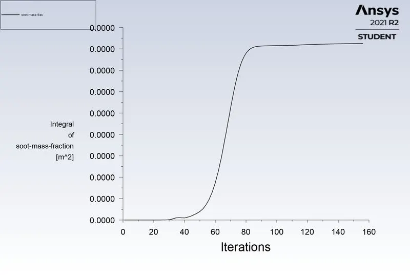
• Integral value reports of Soot and NOx formation has also been parametrized as an output parameter from Report Definitions.
• Once an initial case has been set up for 5 percent water and 95 percent methane case, using parameters, we can run the remaining cases as well.
• Results from the remaining cases have been plotted and images attached in the report.

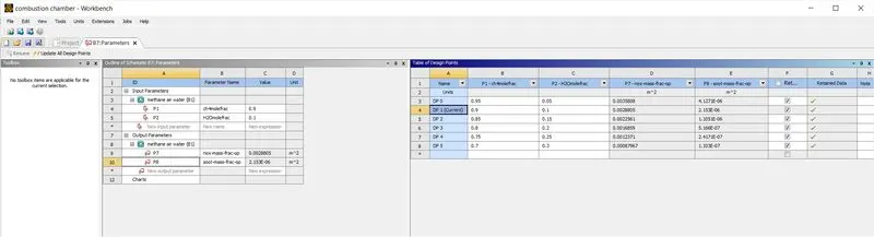
Setting up Parameters

Conclusion

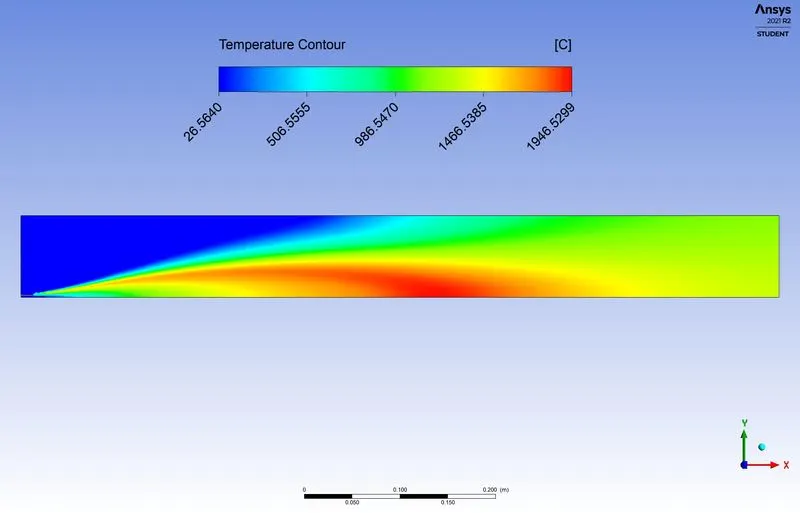
• As mole fraction of water is increased, the NOx and soot formation, which are pollutants and therefore, harmful to the environment, are reduced.
• The peak temperature also in the said cases reduces with an increase in mole fraction of water.
• An integral report definition is used for NOx and soot formation for outlet and internal cells, as an Area Averaged plot will yield a value of almost zero. This is because soot and NOx formations are very scanty across the domain and are localized.
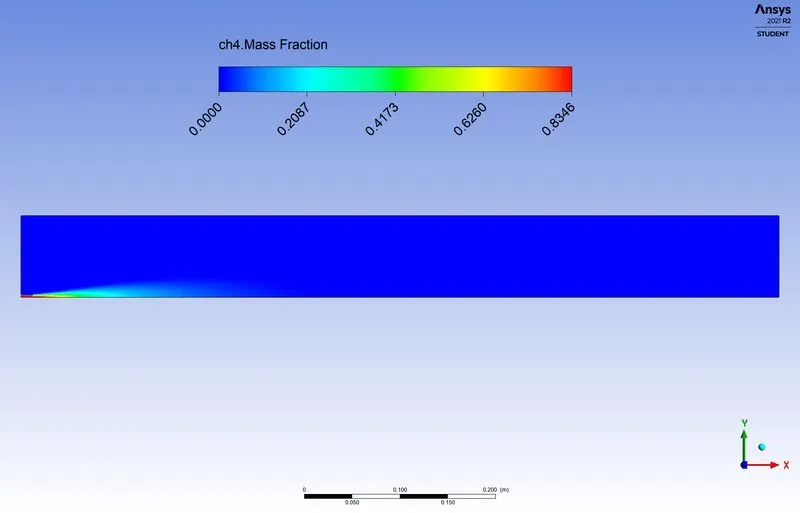
• Mass fraction of Methane falls very rapidly due to combustion of methane into other elementary elements. Turbulence also plays an important role in this particular modelling as non-zero values of turbulent kinetic energy and turbulent dissipation initiate combustion process.
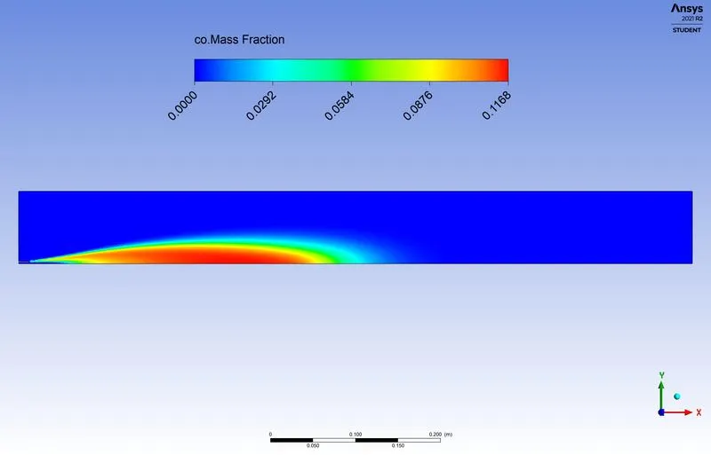
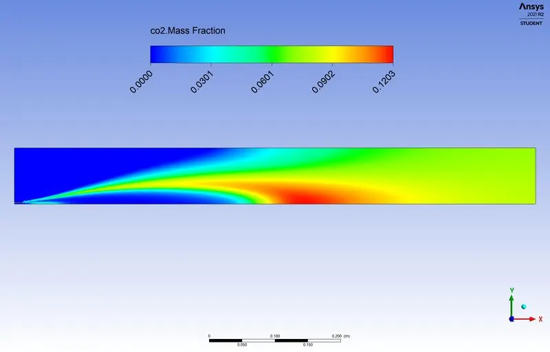
• Carbon dioxide (CO2) mass fraction is zero where carbon mono-oxide (CO) mass fraction is maximum. This can be validated from the second reaction of methane-air-2step reaction mechanism as all the carbon reacts with oxygen to form CO2.
• Nitrogen remains the same across the computational domain with a very slight fall in mass fraction. This slight fall is the amount of radical nitrogen reacting to form NOx pollutant.