Week 3.5 - Deriving 4th order approximation of a 2nd order derivative using Taylor Table method
Aim - Deriving the 4th order approximation of a second-order derivative using the Taylor table method.
The different methods of approximations that have been taken into account in this project are as follows.
1) Central difference scheme in this method is the values of two points from both sides of the reference point that is needed to be found out are taken into the mathematical formula to find out the central differencing schemes.
2) Skewed left-sided difference- To derive skewed left side difference for fourth-order approximation of second order derived by the Taylor table method of finite difference method by using equilibrium below second-order derivative of fourth order approx. The equation to denote the skewed left sided difference is
d^f/dx^2 = af(i)+bf(i-1)+cf(i-2)++df(i-3)+ef(i-4)
3) Skewed right-sided difference- To derive skewd right side difference for fourth order approximation of second order derivative by taylor table method by using the equation given by the following-
d^f/dx^2 = af(i)+bf(i+1)+cf(i+2)+df(i+3)+ef(i+4)
The formula for the central approximation of the second-order derivative are as follows-
d^2/dx^2 = af(i-2)+bf(i-1)+cf(i)+df(i+1)+ef(i+2)
. To find out the central approximation we have to find out the five unknown coefficients and to find out the values we have to use the Taylor table methods .
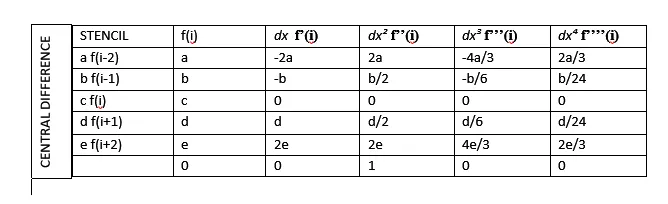
The expansion of the coefficients a , b,c,d and e by central difference is written as follows-
af(i-2) = af(i) - af(i)(2deltax)/1!+ af'(i)(2deltax)^2/2 +af'''(i)(2deltax)^3/3!-af''''(i)(2deltax)^4/4!
This way this template of expansion of the coefficients are used for all other coefficients like a ,b,c,d,e
The picture for taylor's table is as follows-
Code for the fourth-order approximation of second-order derivative of function-
% code to compute 3 different methods of approximation of a fourth order
% for a second order derivative

clear all
close all
% clc
% Assumed value of x and dx

x = pi/3 ;
 dx = linspace(pi/40, pi/4000,20) ;

% given function
analytical_function = exp(x)*cos(x);
analytical_function_derivative = (-2)*exp(x)*sin(x) ;

% central approximation of the fourth order for second order derivative
c_s_approximation = ((-0.08333333333333.*exp(x-2*dx).*cos(x-2*dx)) + (1.3333333333333.*exp(x-dx).*cos(x-dx)) - (2.5.*exp(x).*cos(x)) + (1.3333333333333.*exp(x+dx).*cos(x+dx)) - (0.08333333333333333.*exp(x+(2*dx)).*cos(x+(2*dx))))./(dx.^2) ;

% right side skewed fourth order approx for a second order
R_S_Skewed_Approximation = (((3.75).*exp(x).*cos(x)- ((12.8333333333333).*exp(x+dx).*cos(x+dx))+((17.83333333333333).*exp(x+(2.*dx)).*cos(x+(2.*dx)))-((13).*exp(x+(3.*dx)).*cos(x+(3.*dx)))+((5.083333333333333333).*exp(x+(4.*dx)).*cos(x+(4.*dx))))-((0.83333333333333).*exp(x+(5.*dx)).*cos(x+(5.*dx))))./(dx.^2) ;

% left side skewed fourth order approximation for a second order function
L_S_skewed_Approximation = (((3.75).*exp(x).*cos(x)- ((12.833333333333333333).*exp(x-dx).*cos(x-dx))+((17.8333333333333333).*exp(x-(2.*dx)).*cos(x-(2.*dx)))-((13).*exp(x-(3.*dx)).*cos(x-(3.*dx)))+((5.083333333333333333).*exp(x-(4.*dx)).*cos(x-(4.*dx))))-((0.8333333333333333).*exp(x-(5.*dx)).*cos(x-(5.*dx))))./(dx.^2) ;

% first order approx by using backward approx method
backward_approximation_method = ((exp(x).*cos(x))- (exp(x-dx).*cos(x-dx)))./dx ;

forward_approximation_method =  ((exp(x+dx).*cos(x+dx))- (exp(x).*cos(x)))./dx ;

% error calculation
central_error = abs(analytical_function_derivative- c_s_approximation) ;
R_S_Skewed_error= abs(analytical_function_derivative- R_S_Skewed_Approximation) ;
L_s_skewed_error = (analytical_function_derivative- L_S_skewed_Approximation) ;
forward_approximation_error = abs(analytical_function_derivative-forward_approximation_method) ;
backward_approximation_error= abs(analytical_function_derivative- backward_approximation_method) ;

% making plot

loglog(dx,central_error,'r')
hold on
loglog(dx,R_S_Skewed_error,'b') ;
hold on
loglog(dx,L_s_skewed_error,'g');
hold on
loglog(dx,forward_approximation_error,'y')
hold on
loglog(dx,backward_approximation_error,'k')
legend('central error','right skewed','left skewed','forward approx','backward approx')
xlabel('value of dx')
ylabel('error values')
#) Explanation of the code-
1) We define the variable of x in which we need to find the derivative that is at the point of x = pi/3. and at the step sie or the mesh size is of the dx is created by an 20 equal amount between the pi/40 and the pi/4000.3
2) The second-order analytical derivative of the function is defined and coded and using the value of x the value of the analytical derivative is found.
3) Using the Taylor table that is being defined above we define the coefficient matrix that is A which is defined using the coefficients and the B matrix is defined as the 0 0 1 0 0. Using these the X matrix is found out by iusing the command for X = Inv(A)*B.
4) SO USING THE COEFFICIENTS the central approximation is found out and coded of the second-order derivative of the function.
5) Again by using Taylor's table we find out the coefficients for the right-hand skewed and the left-hand side skewed. and it is coded for the analytical function using the approximation formula. using the proper written coefficients and the proper brackets.
6) The plots are made using the loglog command which helps us to show the rate of change of the error with respect to the mesh size . As the dx changes or increases along the x axis in the y axis the error is plotted.
Skewed scheme attributes compared to the central differences-
1) In central differencing there is a restriction on the number of data points that can be utilized for the computation of the certain points . The number of data points collectively will always ba an odd number mainly due to the fact that the stencil must be symmetric as always. An inequality will cause it to be more skewed this restriction does not exist for skewed schemes.The number of data points considered can be both even and the odd.
2) The usage of a skewed scheme becomes apparent in unidirectional flows.Since a skewed scheme proceeds in one direction only the computation of a single point is that scenario becomes for more accurate as the data points are along a surface. We can calculate heat at a certain point for more accurately mainly because we can take into consideration n different nodes ahead of it. this proves to be an apparant advantage over central differencing.
If central differencing is used in these case it would consider nodes behind the data point as well as in this case the accuracy will decrease as the information it can take from the nodes behind the data points ahead of the main reference point is limited.
3) This is the main use of skewed scheme and for cases like there the skewed scheme can prove to be more accurate.
3) Outcome of the project-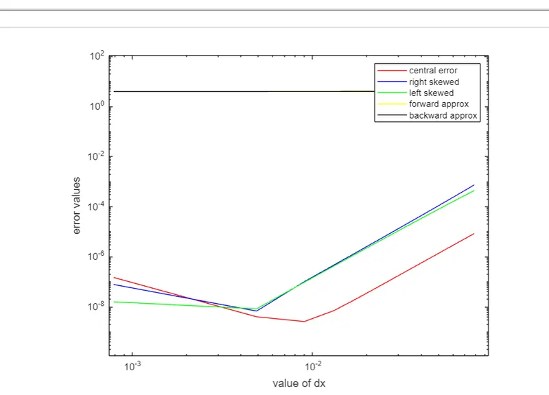
Conclusion - As we are increasing the dx along with the x-axis dx increases then error values decrease and reaches the lowest value for a particular value of dx for the central difference and the left and the right hand skewed and as the value of dx is increased further the error value increases. So as the error value depends on the mesh size or the grid length. As the value of dx increases the error also increases.