Week 4.1 - Genetic Algorithm

AIM of the project - To write a program to code the stalagmite function and to write another code by the help of genetic algorithm(ga), that is inbuilt inside the Matlab to find out the global maxima and global minima of the stalagmite function .

Objectives of the program-

1) To write a code in Matlab to optimize the stalagmite function and find global maxima function.

2) To explain the genetic optimization algorithm(ga) and the syntax of the matlab.

3) To plot the graph of all 3 studies and find the global maxima.

Theory-

Stalagmite - A stalagmite is a type of rock that rises from the floor of a cave due to the accumulation of the material decomposed on the floor. That is why the stalagmite function is given. It is a complex function that is plotted in the Matlab using the function.

Stalagmite and stalactite are mathematical functions that represent geographical features and by that functions, we have to use the genetic algorithm.

To find global maxima we have to first define the stalagmite function-

f(x,y) = f1,x* f2,x* f1,y*f2,y

f1,x = [sin(5.1* pi*x+0.5)]^6

f1,y = [sin(5.1*pi*y+0.5)]^6

f2,x = exp[- 4 * ln(2)*(x-0.0667)^2/0.64]

f2,y = exp[-4*ln(2)*(y-0.0667)^2/0.64]

#) Introduction to Genetic algorithm(ga) -

It is an optimization technique used to solve nonlinear optimization problems.It uses the concept of evolutionary biology to find the global minima of a problem. This algorithm follows the process of natural selection. They help the optimization problem. Genetic algorithms are part of the bigger part of evolutionary algorithms.

It is also used in computer science to find a complex nonobvious solution to algorithmic optimization and search problem.

So to find the global maximum of a function we have to invert the function whose global maximum is to be found , find the minimum value of the inverted function the negative of the global minimum is to be the global maximum of the function.

GA is the method of solving constrained and unconstrained problems base on the natural selection process of evolutionary biology.

Syntax of the ga function - [inputs,fopt] = ga(function , number of variables)

here the number of variables is that is of x and y. Inputs we will get a 1*2 matrix for each iteration, it will basically give the x and y and fopt will give the optimum value of the function containing the x and y as variables.

These variables can be stored and the surf command can ber used to create the surface to visualize the function. we can also use the amrker command to find out the point of the local maximum.

tic and tock command is used to find out the time taken for the iteration to run.

The drawbacks of this study is that since ga command does not know the limits of the x and y . so it can take values more than 0.6 also and the value of x and y can also be less than 0. So to overcome that we need to set up a second study which can put restriction to the value of x and y .Hence we set up upper and lower bounds for the ga function and the synatax is of

[inputs,fopt] = ga(function,number of variables A, b,Aeq,beq,lb,ub) where lb is the lower bound and the ub is of upper bounds.

A- linear inequality constraints.

b - linear inequality constraints

Aeq - linear equality constraints

beq- linear equality constraints.

Code for the genetic approximation(Ga)-

 clear all
close all
clc
x=linspace(0,0.6,150);
y=linspace(0,0.6,150);
num_space= 50 ;

% forming 2D array
[xx,yy]= meshgrid(x,y);
for i=1: length(xx)
    for j=1:length(yy)
        input_vector(1)=xx(i,j);
        input_vector(2)=yy(i,j);
        f(i,j)= stalagmite(input_vector) ;
    end
end

        % initiating ga
        tic
        for i=1:num_space
            [results,fopt(i)]=ga(@stalagmite,2);
            xopt(i)= results(1);
            yopt(i)= results(2);
        end
        study_time1=toc;
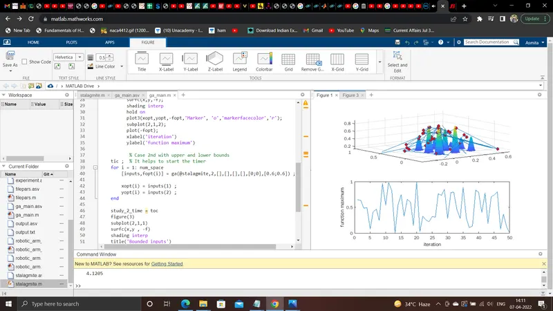
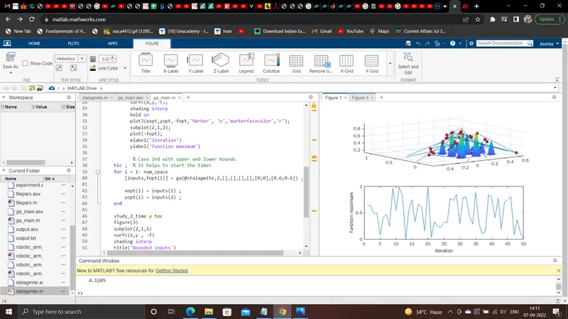
        figure(1)
        subplot(2,1,1)
        surfc(x,y,-f);
        shading interp
        hold on
        plot3(xopt,yopt,-fopt,'marker','o', 'markerfacecolor','r');
        subplot(2,1,2);
        plot(-fopt);
        xlabel('iteration')
        ylabel('function maximum')

         % Case 2nd with upper and lower bounds
  tic ;  % It helps to start the timer 
  for i = 1: num_space
      [inputs,fopt(i)] = ga(@stalagmite,2,[],[],[],[],[0;0],[0.6;0.6]) ;

      xopt(i) = inputs(1) ;
      yopt(i) = inputs(2) ;
  end

  study_2_time = toc 
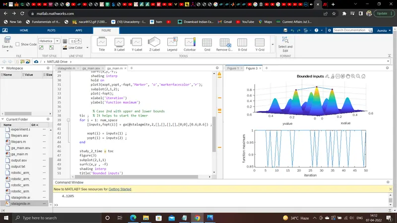
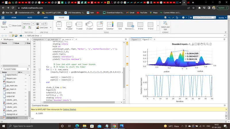
  figure(3)
  subplot(2,1,1)
  surfc(x,y , -f)
  shading interp 
  title('Bounded inputs')
  xlabel('xvalue')
  ylabel('yvalue')
  hold on
  plot3(xopt,yopt,-fopt,'Marker', 'o', 'markersize',4,'markerfacecolor','r');
  subplot(2,1,2)
  plot(-fopt)
  xlabel('iteration')
  ylabel('function maximum')

#) explanation of the code-

1) The linspace command is used to create the dimensions in the two directions in the x and the y axis from 0 to 0.6 and crating 150 divisions between them.

2) Then the two dimensional array is created using the meshgrid by combining the x and the y axis .

3) Now we have to use the two for loops we have to extend the two loop counters i and j and we have to vary it for the entire length xx and the yy axis. We store the values of the instance at the input_vector(1) and in the input_vector(2).

4) Then the function f(i,j) is of the stalagmite function and we have coded the stalagmite function separately which has the inputs as the (input_vector) .

5) Then we have to initiate or call the genetic algorithm optimization solver and we use the for loop for the entire num_space

we use the inputs as ga(@stalagmite,2).

6) The output is named the xopt and yopt this is the optimum coordinates of the points where the function is at the global maxima. The ga solver actually gives the output as the xopt nad the yopt.

7) Now in the second part we do the study by including the limits of the x and y axis. Now the new syntax for the ga or geentic algorithm is of [inputs,fopt] = ga(function,number of variables A, b,Aeq,beq,lb,ub) .

8) Then the subplot is created and the surface is created by including the engative of the function that is of -f.

The syntax is of surfc(x,y,-f).

9) Plot number 3 is also plotted of the second code using the bounded points and the stalagmite function using the markers as 'o' , markersize of 4 is also included and the markerfacecolor of red is used. plot of -foptimum is given and the xlabel and the ylabel is given for the function plot.

#) Code of the stalagmite function

function  [f] =stalagmite(input_vector)
x= input_vector(1);
y= input_vector(2);
f1=(sin(5.1*pi*x+0.5)).^6;
f2=exp((-4*log(2)*((x-0.0667).^2))/0.64);
f3=(sin(5.1*pi*y+0.5)).^6;
f4=exp((-4*log(2)*((y-0.0667).^2))/0.64);
f =-(f1*f2*f3*f4);
end

1) A function code is created by the name of stalagmite function as the inputs of the (input_vector).

2) The x and y of teh function is as of x= input_vector(1) and y = input_vector(2).

3) The entire stalagmite function is divided into 4 parts of the functions f1, f2 ,f3 and the f4.

4) The function f is of the negative of the multiplication of the four functions.

Outputs of the code-

For the first part of the code the outpur function plot -

1)

2)

3) The function plots of bounded points

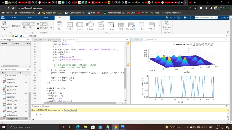
4)

5) The co-ordinates of the global maxima is of-

#) Problems faced in the project-

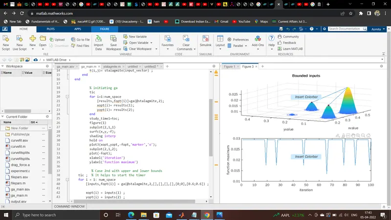
1) Wrong coding of the stalagmite function because the bracket was not given correctly. So wrong function was plotted. then the bracket was adjusted.

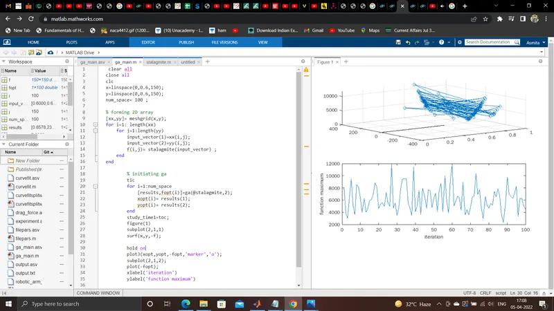
2) Wrong coding of function-

#) the study time of the project is found out and printed in the command window = 4.12 seconds for the entire iterations of 5o.

#) Conclusions-

The different studies of global approximations of the stalagmite function is done and the plots are also made .The co-ordinates of the global maxima are also found of x and y is also found out.

The time period of the study is also found out.