Week 5 - Rayleigh Taylor Instability
Aim - To conduct the RT CFD simulation
Introduction- RTI is a phenomenon that occurs on the interface of fluids of different density wherein the lighter fluids push the heavier fluid due to the density difference. It is a dynamic process wherein the system tries to reduce its combined potential energy.
Theory - Initially the system is in the hydrodynamic stability in which the heavier fluid is sitting at the top of the lighter fluid in a constant gravitational field . As the RTI develops the initial development is in the form of the linear growth phase ,In the first stage, the perturbation amplitudes are small when compared to their wavelengths, and the equations of motion can be linearized, resulting in exponential instability growth. In the early portion of this stage, a sinusoidal initial perturbation retains its sinusoidal shape. However, after the end of this first stage, when non-linear effects begin to appear, one observes the beginnings of the formation of the ubiquitous mushroom-shaped spikes (fluid structures of heavy fluid growing into light fluid) and bubbles (fluid structures of light fluid growing into heavy fluid). The growth of the mushroom structures continues in the second stage and can be modeled using buoyancy drag models, resulting in a growth rate that is approximately constant in time. In the non linear it is not possible to neglect the nonlinearity in the system. In general the density disparity between fluids will determine the structure of the non linear terms instability flows(assuming the viscosity and surface tension is negelcted).
Examples include supernova water suspended atop, oil mushroom clouds formed due to volcanic erruption.
CFD models based on mathematical analysis of Rayleigh Taylor instability-
1)Mass diffusion model- The mass diffusion equation the transport of mass and energy due to the model viscosity and hence drives the actual mixing in the fluids even if any configuration is Rayleigh Taylor unstable the diffusion process could be responsible for mixing if the viscosity is large.
2) Single fluid model-
1) Potential flow modeel- This model is valid for all instability from the linear stage through the non linear to the asymptotic but limited to the Atwood number = 1 . In this model the single mode perturbation expands the flow equation to the second order around the bubble tips. Hence obtaining an ODE for bubble velocity.
2) Buoyancy drag model - It is the valid for every atwood number but limited to the non linear stage of the instability. It uses the ordinary differential equation to evolve the width of the mixing layer. The bubble or spike amplitudes are described by balancing the inertia, buoyancy and drag force. These model can not model the mixing interface. can not be easily extended to the 2 or 3 dimensional as a rule do not address demixing , also known as counter gradient approach that is reduction of the total fluid mass within the mixing zone. To address these problems two model fluid is used or multi phase model is used.
3) Besnard - Harlow - Rauenzahn (BHR) - It is the more advanced version of the single phase fluid . The BHR model is based on the evolution equation arising from the second-order correlation and the gradient diffusion approximation. Using a mass averaged decomposition the original BHR equation includes full transport equation for the transport equation. Turbulent mass flux ,velocity and density fluctuations and the turbulene kinetic energy dissipation rate.
3) Multi fluid model - These model use a separate equations for each fluid in addition to the main flow equations and provide an accurate framework for modelling framework for demixing by capturing the relative motion of the different fluid fragments
The first step of the turbulence model is to perform the Reynolds averaging of the Navier Stokes equations and the resultant terms.
Two equation K-l turbulence model- The k-l turbulence model involves an equation for the turbulent kinetic energy and turbulent length scale of L . The starting point deriving the model equation is the buoyancy drag capability for the similar growth of R-T instabilities.
Three equation k-l-a turbulence model- The three equation model is an advancement of the k-l turbulence model including a third equation for the turbulent mass flux velocity.
Four equation k - l -a-b turbulence model - The four equation model was an advancement of the k-l turbulence model including a fourth model for the density specific volume covariance. The model can accurately reflect the changes in the density fluctuation.
#) The design of the model was made in the spaceclaim-
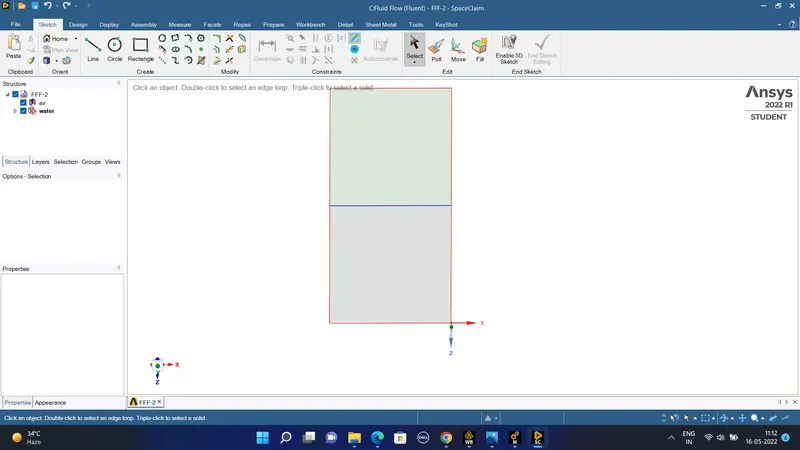
The spaceclaim geometry was made by the rectangle geometry option here we are to make a square of the dimension of 20 mm and the pull tool is used to make the two-dimensional geometry into a surface . Then a new sketch option was used again to make another rectangle was made on top of it to simulate another medium of fluid containing a fluid of heavier density.
The share topology option is used to share the geometry from SpaceClaim to the mesh .
The mesh was created by giving the proper element size which is less than the normal automatically generated mesh
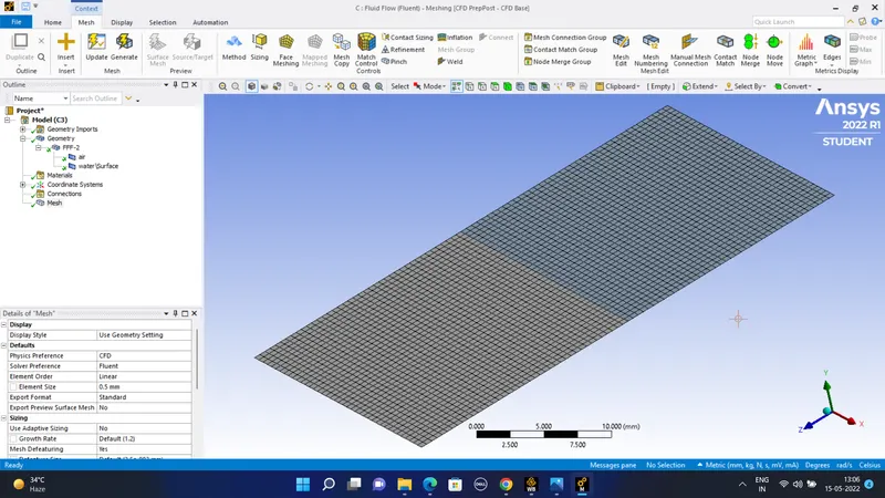
The element size = 0.5 mm
Then the fluent solver is used to solve the Rayleigh- Taylor instability and the settings were made for the mutiphase flows
The laminar flow solver is used to create the simulation and the two material one is of air and the other material is of the water in the liquid stage.
#) The multi phase model is used to cater to the number of Eulerian phase of 2 the Homogenous model of volume of fluid is used . In the volume fraction parameter implicit method is used .
The solution method is of SIMPLE algorithm is used for the solution.
The patch is done for the different material of air and water for water the value given is of 1 and for the gas it is of 0
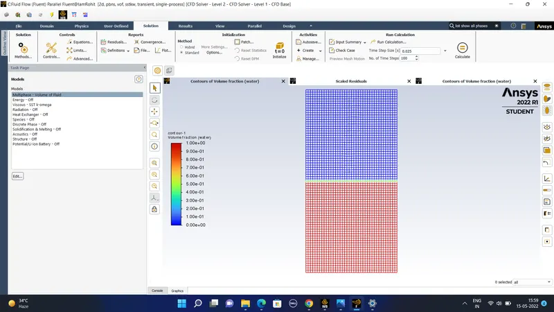
The residuals and the results obtained are-
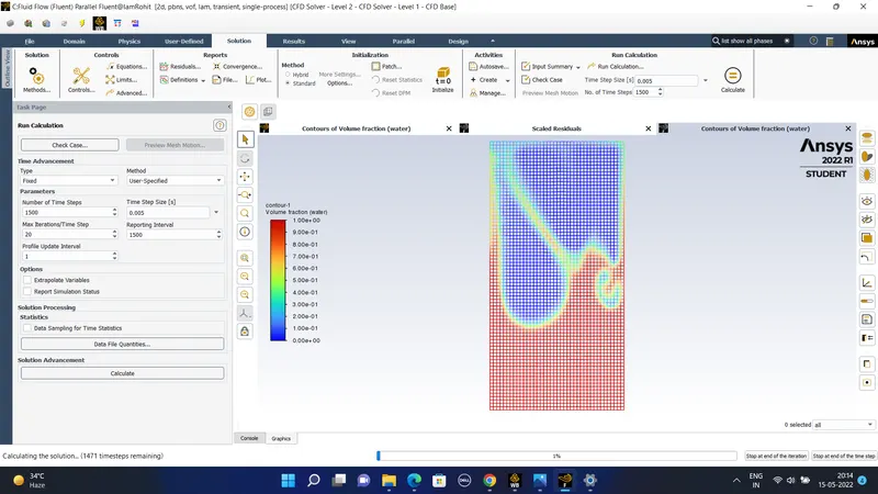
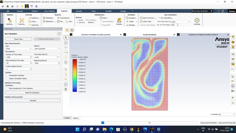
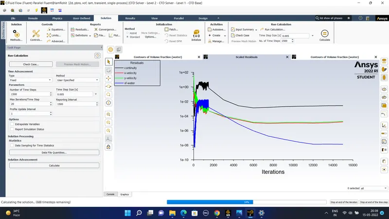
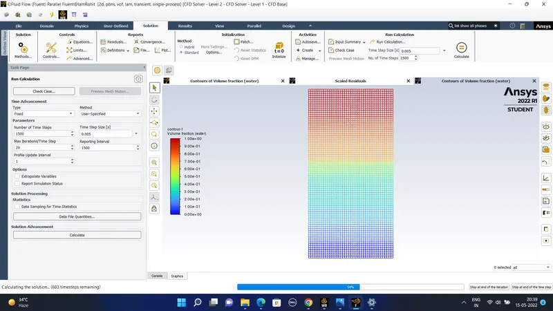
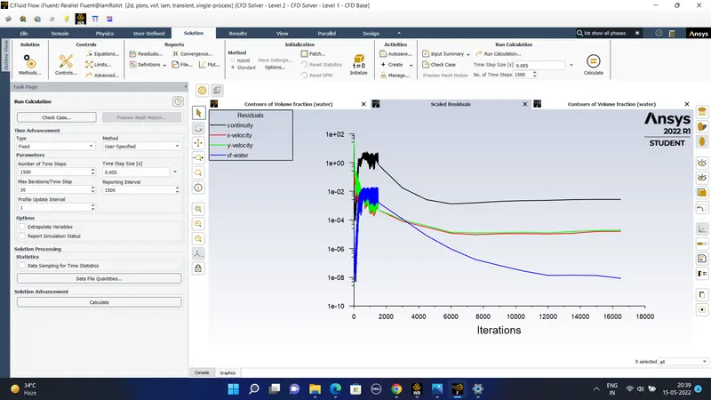
The final contour of the simulation and the residuals obtained are-
#) The animation obtained from the coarse mesh would be of - https://drive.google.com/file/d/183q0MbPDuKvXiDfOPPNxPtyN-TyOuEOI/view?usp=sharing
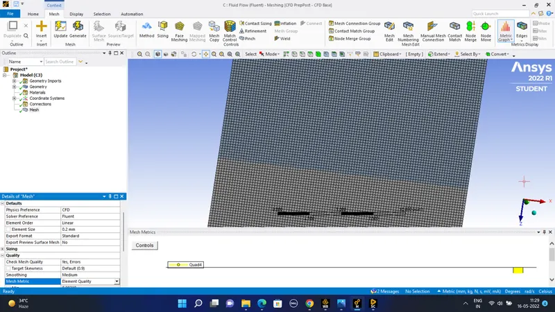
The Finer mesh was done in which the mesh element size was reduced to the 0.2 mm
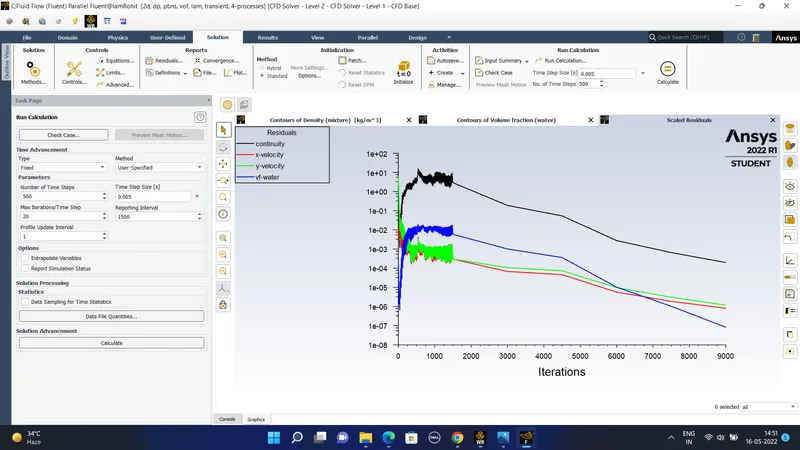
The residuals obtained are-
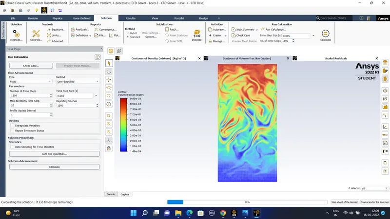
The animation for the finer mesh -
https://drive.google.com/file/d/1KS1-ztMa5OLoj04E9hNyQ_bxILmQ1c5d/view?usp=sharing
case3) Now we are using the user-defined material and the water so this leads to a new simulation the animation is also created separately and saved for use-
The residuals obtained are-
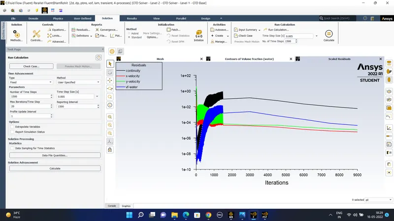
The contour obtained after 500 iterations and giving the time step = 0.005 sec- The google drive link for the animation video.
https://drive.google.com/file/d/1fkbWRwx2ec0Lwx5PZHsByB0apkL6zn1D/view?usp=sharing
#) Atwood number -
The Atwood number (A) is a dimensionless number in fluid dynamics used in the study of hydrodynamic instabilities in density stratified flows. It is a dimensionless density ratio defined as

where
 = density of heavier fluid
 = density of the lighter fluid.
- Atwood number is an important parameter in the study of Rayleigh- Taylor instabilities.
rho1 = 998.2 kg/m^3
rho2 = 1.2 kg kg/m^3
so the
A = (998.2-1.22)/(998.2+1.22) = 0.428
Behaviour of RT instability on variation of the Atwood number - RTI involves in three different stages linear stability, mushroom head or bubble rising formation long term evolution due to bubble merging and mixing . For a low Atwood number mushroom head shape is relatively symmetrical , the disturbance or perturbations are linear for a larger term. In contrast for the large Atwood number bubble and mushroom shape is less symmetrical also it occurs at an accelerating time which leads to nonlinear growth.
#) Conclusions - 1) With the finer mesh of size of 0.2 mm we can get to capture the instability and its distribution in a much more accurate manner . Though with the finer mesh it takes much more time to attain the correct results of settling but with higher accuracy.
2) SInce the instabilities are very much haphazard and it is changing in an unpredictable manner so we require to use the transient solver better accuracy than the steady state solver.