Week 7 - Simulation of a 1D Super-sonic nozzle flow simulation using Macormack Method

AIM- To simulate the isentropic flow through a quasi 1 - D subsonic nozzle by deriving both the conservation and nonconservation form of the governing equation and solve them by implementing te Macormack method in the MATLAB .

Problem statement-

Determine the steady -state temperature distribution for the flow field variables and to investigate the difference between the two forms of the governing equations by comparing their solutions and making plots.

1) Steady-state distribution of primitive variable inside the nozzle.

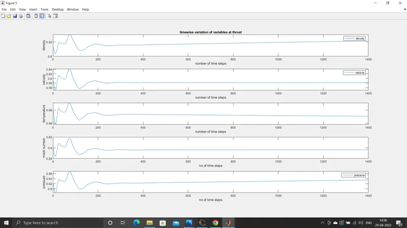
2) Time-wise or the time-dependent variation of a primitive variable.

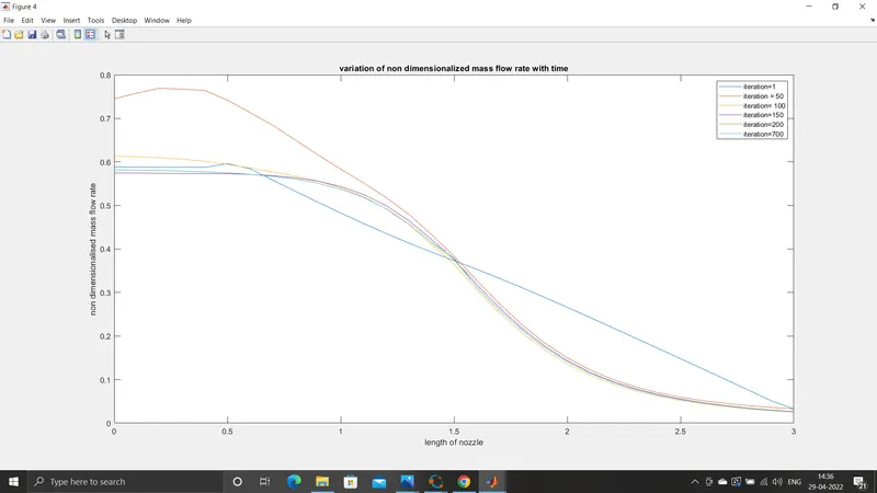
3) Variation of mass rate distribution inside the nozzle at different times using the time marching methods.

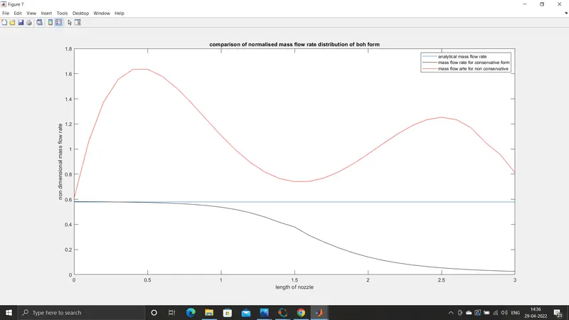
4) Comparison of the normalized mass flow rate distribution of both forms.

#) Theory of the Nozzle and Maccormack method-

Any numerical solution of the isentropic flow through a 1-D SUBSONIC - SUPERSONIC NOZZLE IS UNREasonable , while an analytic solution exists for this kind of problems. However we are trying here to establish the broadened capability of CFD . Here we implement both the numerical solution for the conservative and the non-conservative forms both.

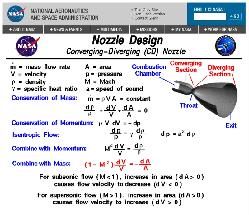
A nozzle is used to accelerate hot exhaust to produce thrust as described by Newton's law. A nozzle is a relatively simple device, just a specially shaped tube through which hot gases flow. Rockets typically use a fixed convergent section followed by a fixed divergent section for the design of the nozzle. This nozzle configuration is called a convergent-divergent, or CD, nozzle. In a CD rocket nozzle, the hot exhaust leaves the combustion chamber and converges down to the minimum area, or throat, of the nozzle. The throat size is chosen to choke the flow and set the mass flow rate through the system. The flow in the throat is sonic which means the Mach number is equal to one in the throat.

the differential form of the equation governing nozzle gas flow-

Macormack method- In Computational Fluid dynamics, the MacCormack method is a widely used discretization scheme for the numerical solution of hyperbolic partial differenial equations This second-order finite difference method was introduced by Robert W. MacCormack in 1969. The MacCormack method is elegant and easy to understand and program.

The macormack method consistes of two steps which occure simultaneously one is called the predictor step and the second is the corrector step. The detailed procedure are as follows-

The application of MacCormack method to the above equation proceeds in two steps; a predictor step which is followed by a corrector step.

Predictor step: In the predictor step, a "provisional" value ou at time level u estimated as follows

The above equation is obtained by replacing the spatial and temporal derivatives in the previous first order hyperbolic equation using forward differences.

Corrector step: In the corrector step, the predicted value is corrected according to the equation

Note that the corrector step us backward finite differences approximations for spatial derivative. The time-step used in the corrector step is in contrast to the {\displaystyle \Delta t} used in the predictor step.

Replacing the term by the temporal average

to obtain the corrector step as

Governing equation are marched in terms of PDE for both forms to use Time marching problem solution for the problem THESE REPRESENT in numerical aspect only

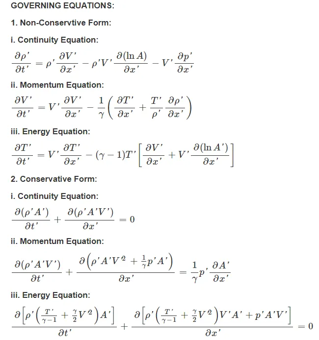
The Governing equation in the non-conservative and the conservative forms are as follows-

Non - dimensionless quantities-

Temperature ratio = T' = T/To .

Densiy ratio = rho / rho o .

non dimensianl distance = x' = x/L , L is the length of the nozzle.

non dimensional time = t' = (t/L/ao)

non dimensional area A' = (A/A*) A* is the sonic throat area.

Macormack method is used for non linear equation(inviscid Burgers equation, Euler equation). For non-linear equation it provides the best result. For linear equation Lax-Wendroff method is used.

The main code for the supersonic nozzle flow code-

% matlab main code for supersonic nozzle
clear all
close all
clc

% defining dimensional mesh size
L = 3 ;
n = 31 ;
x = linspace(0,3,n) ;
dx = x(2)-x(1) ;
gamma = 1.414 ;
% CFL criteria
c = 0.5 ;

% time steps
nt = linspace(1,1400,1400) ;

% calculate initial profile
rho = 1-0.3146*x ;
T = 1-0.2314*x ;
v = (0.1+1.09*x).*T.^0.5 ;
a = 1+2.2*(x-1.5).^2 ;

% writing function for non- conservative form
[mfr_analytical,mfr_e] = nonconservative(x,L,n,gamma,nt);
[mfr_con]= conservative(x,L,n,gamma,nt) ;

figure(7);
plot(x,mfr_analytical)
hold on
plot(x,mfr_con,'k')
hold on
plot(x,mfr_e,'r')
xlabel('length of nozzle')
ylabel('non dimensional mass flow rate')
legend('analytical mass flow rate ','mass flow rate for conservative form','mass flow arte for non conservative')
title('comparison of normalised mass flow rate distribution of boh form')

Now two separate function codes are being created to code separately the governing equations of the conservative and the non conservative equations using their own physics and the finite difference is carried out for both of the conservative and the non conservative form by the Maccormack method that proves perfect for the inviscid supersonic flow because in this range the governing equations behave slike the hyperbolic equations.

#) Function code for the non-conservative form

% The function code for nthe non conservative governing equation
% Code to solve the 1-D SUPERSONIC nozzle flow by Macormack method
function[mfr_analytical,mfr_e]= nonconservative(x,L,n,gamma,nt)



% Inputs to the problem
L = 3 ;
n = 31 ;
x = linspace(0,L,n) ;
dx = x(2)-x(1) ;
gamma = 1.414;

% calculate initial progile
mfr_analytical =0.579*ones(1,n) ;
rho = 1-0.3146*x ;
T = 1-0.2314*x ;
v = (0.1+1.09*x).*T.^0.5 ;
a = 1+2.2*(x-1.5).^2 ;
c = 0.5 ;
mfr_initial = rho.*a.*v ;
M_initial = v./T.^0.5 ;
p_initial = rho.*T ;
% calculating throat value
throat = find(a==1) ;

% time steps
nt = linspace(1,1400,1400) ;
dt = min((c*dx)./((sqrt(T)+v))) ;
number_iter = 0 ;

% starting time loop
tic ;
for k = 1:nt
    % predictor method
    rho_old = rho ;
    v_old = v ;
    T_old = T ;
    for j = 2:n-1

        dvdx = (v(j+1)-v(j))/dx ;
        drhodx = (rho(j+1)-rho(j))/dx ;
        dTdx = (T(j+1)-T(j))/dx ;
        dlogadx = (log(a(j+1))-log(a(j)))/dx ;

       

        % continuity equation
        drhodt_p = -rho(j).*dvdx-rho(j).*v(j).*dlogadx-v(j).*drhodx ;

         % momentum eqyation
        dvdt_p = -v(j).*(dvdx)-(1/gamma).*(dTdx+(T(j)/rho(j))*drhodx);

        % energy equation
        dTdt_p = -v(j)*dTdx-(gamma-1)*T(j)*(v(j)*dlogadx) ;

        % solution update
        v(j) = v(j)+(dvdt_p*dt) ;
        rho(j)= rho(j)+(drhodt_p*dt) ;
        T(j)= T(j)+dTdt_p*dt;
    end


% corrector method
 for i = 2:n-1

        dvdx = (v(i)-v(j-1))/dx ;
        drhodx = (rho(i)-rho(i-1))/dx ;
        dTdx = (T(i)-T(i-1))/dx ;
        dlogadx = (log(a(i))-log(a(i-1)))/dx ;

       

        % continuity equation
        drhodt_c = -rho(i).*dvdx-rho(i).*v(i).*dlogadx-v(i).*drhodx ;

         % momentum eqyation
        dvdt_c = -v(i).*(dvdx)-(1/gamma)*(dTdx+(T(i)./rho(i)).*drhodx);

        % energy equation
        dTdt_c = -v(i).*dTdx-(gamma-1).*T(i).*(dvdx+v(i).*dlogadx) ;

       
    end
% compute the average time derivative
drhodt(i) = 0.5*(drhodt_p+drhodt_c) ;
dvdt(i) = 0.5*(dvdt_p+dvdt_c) ;
dTdt(i) = 0.5*(dTdt_p+drhodt_c) ;

% final solution update
for i = 2:n-1
    rho(i)= rho_old(i)+drhodt(i).*dt ;
    v(i)= v_old(i)+dvdt(i).*dt ;
    T(i)= T_old(i)+dTdt(i).*dt;
end
% apply the boundary conditions
v(1)= 2*v(2)-v(3) ;
rho(1) = 1 ;
t(1)= 1 ;

% outlet boundary condition
v(n) = 2*v(n-1)-v(n-2) ;
rho(n) = 2*rho(n-1)-rho(n-2);
T(n) =2*T(n-1)-T(n-2) ;

% primitive variables at exit

p_e =rho.*T;
M_e= v./T.^0.5 ;
mfr_e = rho.*a.*v;

%  primitive values at the throat
p_e = rho.*T ;
M_e = v./T.^0.5 ;
mfr_e = rho.*a.*v ;

% values at the throat values
mfr_throat(k) = mfr_e(throat) ;
p_throat(k) = p_e(throat);
v_throat(k) = v(throat) ;
rho_throat(k)= rho(throat) ;
T_throat(k) = T(throat) ;
M_throat(k)= M_e(throat) ;

figure(1)
if(number_iter==1)
    plot(x,mfr_e)
    hold on
elseif(number_iter==50)
    plot(x,mfr_e)
    hold on
elseif(number_iter==100)
    plot(x,mfr_e)
    hold on
elseif(number_iter==150)
    plot(x,mfr_e)
    hold on
elseif(number_iter==200)
    plot(x,mfr_e)
    hold on
elseif(number_iter==700)
    plot(x,mfr_e)
    hold on
elseif(number_iter==1400)
    plot(x,mfr_e)
    hold on
    xlabel('length of nozzle')
    ylabel('non dimensional mass flow rate')
    legend('number iter==1','number iter==50','number iter==100','number iter==200','number iter==700','number iter==1400','mfr analytical','mfr initial')
    title('variation of the non dimensional mass flow rate along the length of the nozzle with varying the time step')
end
end
compuational_time = toc ;
figure(2)
subplot(5,1,1)
plot(nt,p_throat)
xlabel('number of time steps')
ylabel('density')
legend('density at throat')
subplot(5,1,3)
plot(nt,T_throat)
xlabel('number of time steps')
ylabel('temperature')
legend('temperature at throat')
subplot(5,1,4)
plot(nt,v_throat)
xlabel('number of time steps')
ylabel('velocity')
legend('velocity at throat')
subplot(5,1,5)
plot(nt,M_throat)
xlabel('number of time steps')
ylabel('mach number')
legend('velocity at throat')
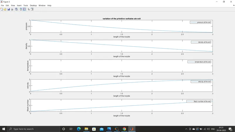
figure(3)
subplot(5,1,1)
plot(x,p_e)
xlabel('length of the nozzle')
ylabel('pressure')
legend('pressure at the exit')
title('variation of the primitive varibales ate exit')
subplot(5,1,2)
plot(x,rho)
xlabel('length of the nozzle')
ylabel('density')
legend('density at the exit')
subplot(5,1,3)
plot(x,t)
xlabel('length of the nozzle')
ylabel('temperature')
legend('temperature at the exit')
subplot(5,1,4)
plot(x,v)
xlabel('length of the nozzle')
ylabel('velocity')
legend('velocity at the exit')
subplot(5,1,5)
plot(x,M_e)
xlabel('length of the nozzle')
ylabel('Mach number')
legend('Mach number at the exit')
end

#) the function code for the conservative form of the governing equations-

% function code for conservative governing equations
function [mfr_con] = conservative(x,L,n,gamma,nt)

% defining other input parameters
gamma = 1.4 ;
L = 3;
n = 31 ;
x = linspace(0,L,n) ;
dx = x(2)-x(1) ;

rho = 1-0.3146*x ;
T = 1-0.2314*x ;
v = (0.1+1.09*x).*T.^0.5 ;
a = 1+2.2*(x-1.5).^2 ;
% throat
throat= find(a==1) ;
c = 0.5 ;

% initializing temperature and the density

for i = 1:length(x)
    if x(i)>=0 && x(i) <0.5
        rho_con(i) = 1 ;
        temp_con(i) = 1 ;

    elseif x(i)>=0.5 && x(i)<1.5
        rho_con(i) = 1 - (0.366.*(x(i)-0.5)) ;
        temp_con(i) = 1- (0.167.*(x(i)-0.5)) ;

    elseif x(i)>=1.5 && x(i)<=3
        rho_con(i)= 0.634-(0.3879.*(x(i)-1.5)) ;
        temp_con(i) = 0.833-(0.3507.*(x(i)-1.5)) ;

    end
end

% calculating primitive variables
v_con = 0.59./(rho_con.*a) ;
p_con = rho_con.*temp_con ;

% calculating solution vector
U1 = rho_con.*a ;
U2 = rho_con.*a.*v_con ;
U3 = rho_con.*a.*((temp_con)/(gamma-1)+(0.5*gamma*v_con.^2)) ;
nt = linspace(1,1400,1400) ;
tic ;

iteration = 0 ;
% time iteration usinf for loop for the entire time step
for k = 1:length(nt)
% prdeictor step
    % Creating copy of solution vector
    U1_old = U1 ;
    U2_old = U2 ;
    U3_old = U3 ;

    % calculating dt
    dt_con = min((c*dx)./((sqrt(temp_con)+v_con))) ;

    % calculation of  flux vector
    F1 = U2 ;
    F2 =(U2.^2./U1)+((gamma-1)/gamma)*(U3-((gamma/2)*(U2.^2./U1))) ;
    F3 = (gamma*U2.*U3./U1)-(gamma*(gamma-1)/2)*(U2.^3./U1.^2) ;

    % calculating source term
    for j = 2:n-1
        J2(j) = (rho_con(j).*temp_con(j).*(a(j+1)-a(j)))/(gamma*dx) ;
        dU1dt_p(j) = -(F1(j+1)-F1(j))/dx ;
        dU2dt_p(j) = -(F2(j+1)-F2(j))/(dx)+J2(j) ;
        dU3dt_p(j)=-(F3(j+1)-F3(j))/dx ;
        % updating values
        U1(j) = U1(j)+(dU1dt_p(j)*dt_con) ;
        U2(j)= U2(j)+(dU2dt_p(j)*dt_con) ;
        U3(j)= U3(j)+(dU3dt_p(j)*dt_con) ;
    end

    % Updating the primitive values
    rho_con = U1./a ;
    v_con = U2./U1;
temp_con = (gamma-1)*(U3./U1-(gamma/2)*v_con.^2) ;
p_con = rho_con.*temp_con ;

    % updating  flux vector
    F1 = U2 ;
    F2 = (U2.^2./U1)+((gamma-1)/gamma)*(U3-((gamma/2)*(U2.^2./U1))) ;
    F3 = (gamma*U2.*U3./U1)-(gamma*(gamma-1)/2)*(U2.^3./U1.^2) ;

    % corrector step
     for j = 2:n-1
         J2(j)= (rho_con(j).*temp_con(j).*(a(j)-a(j-1)))/(gamma*dx) ;
         dU1dt_c(j) = -(F1(j)-F1(j-1))/dx ;
         dU2dt_c(j) = -(F2(j)-F2(j-1))/(dx)+J2(j) ;
         dU3dt_c(j)= -(F3(j)-F3(j-1))/dx ;
     end

     % average time step value
     dU1dt_a = 0.5*(dU1dt_c+dU1dt_p) ;
     dU2dt_a =0.5*(dU2dt_p+dU2dt_c) ;
     dU3dt_a = 0.5*(dU3dt_c+dU3dt_p) ;

     for j = 2:n-1 
         U1(j) = U1_old(j)+(dU1dt_a(j)*dt_con) ;
         U2(j) = U2_old(j)+(dU2dt_a(j)*dt_con) ;
         U3(j)=U3_old(j)+(dU3dt_a(j)*dt_con) ;
     end

     iteration =iteration+1 ;

     % left boundary condition declaration
     U1(1)= rho_con(1).*a(1) ;
     U2(1)= 2*U2(2)-U2(3) ;
     U3(1)= U1(1)*(temp_con(1)./(gamma-1)+(gamma/2)*v_con(1).^2 );

     % right boundary conditions
      U1(n)= 2*U1(n-1)-U1(n-2) ;
     U2(n)= 2*U2(n-1)-U2(n-2) ;
     U3(n)= 2*U3(n-1)-U3(n-2) ;

     % calculating primiive variables
     rho_con = U1./a ;
     v_con = U2./a ;
     temp_con = (gamma-1)*(U3./U1-(gamma/2)*v_con.^2);
     p_con = rho_con.*temp_con;
     mfr_con = rho_con.*v_con.*a ;
     M_con = v_con./temp_con.^0.5 ;

     % calculating throat values
     rho_con_throat(k) = rho_con(throat) ;
     temp_con_throat(k)= temp_con(throat);
     v_con_throat(k)= v_con(throat) ;
     mfr_con_throat(k)= mfr_con(throat);
     M_con_throat(k) = M_con(throat) ;
     p_throat(k) = p_con(throat) ;

     % calculating mass flow rate
     mfr(iteration,:)=rho_con.*a.*v_con ;
end
computatational_time = toc ;

% plotting figures
figure(4);
plot(x,mfr(1,:))
hold on
plot(x,mfr(50,:))
hold on
plot(x,mfr(150,:))
hold on
plot(x,mfr(200,:))
hold on
plot(x,mfr(700,:))
hold on
plot(x,mfr(1400,:))
hold on
xlabel('length of nozzle')
ylabel('non dimensionalised mass flow rate')
legend('iteration=1','iteration = 50','iteration= 100','iteration=150','iteration=200','iteration=700','iteration=1400')
title('variation of non dimensionalized mass flow rate with time')

figure(5)
subplot(5,1,1)
plot(nt,rho_con_throat)
xlabel('number of time steps')
ylabel('density')
legend('density')
title('timewise variation of variables at throat')
subplot(5,1,2)
plot(nt,v_con_throat)
xlabel('number of time steps')
ylabel('velocity')
legend('velocity')
subplot(5,1,3)
plot(nt,temp_con_throat)
xlabel('number of time steps')
ylabel('temperature')
subplot(5,1,4)
plot(nt,M_con_throat)
xlabel('no of time steps')
ylabel('mach number')
subplot(5,1,5)
plot(nt,p_throat)
xlabel('no of time steps')
ylabel('pressure')
legend('pressure')

figure(6)
subplot(5,1,1)
plot(x,rho_con)
xlabel('legth of nozzle')
ylabel('density')
legend('density')

subplot(5,1,2)
plot(x,v_con)
xlabel('length of nozzle')
ylabel('velocity')
legend('velocity')
subplot(5,1,3)
plot(x,temp_con)
xlabel('length of nozzle')
ylabel('temperature')
legend('temperature')

subplot(5,1,4)
plot(x,p_con)
xlabel('length of nozzle')
ylabel('pressure')
legend('pressure')

subplot(5,1,5)
plot(x,M_con)
xlabel('length of nozzle')
ylabel('mach number')
legend('mach number')
end

#) Explanation of the code-

1) In the non conservation code since the continuity , momentum and the enrgy equations are large. We dive it into 4 small parts . Then we code for the main governing equations.

2) Then the algorithm for the predictor an dthe corrector steps are followed in the predictor the slope of the quantities like density, velocity and teh temperature is found out at thr i th node at the time step of t using the forward difference technique.

3) To find the value of the variables at the next time step (t+deltat) we update it with the help of linear extarpolation.

4) Next in the corrector step we use the backward difference to find the slope at the next time step that is (t+deltat).

In the corrector time derivative we use the updated value of the density,velocity and temperature

Then the average slope gradient is calculated by considering the corrector an dthe predictor step data. finally the value of the quantities rho, Velocity and Temperature is found out at the next time step of (t+deltat).

5) The entire length of the nozzle or domain is divided into 1400 equal equal parts these would form the mesh inside the length of the nozzle. The time step dt is created by the formula provided in the code. The entire code is run for the total time step of nt = 1400 using a for loop.

6) The space loop is run for the entire domain except for the boundary nodes because value is known at that points.

7) Next the boundary conditions are declared for the left running boundary and the right running boundary.

The code then moves to the next time step this updated or new value is obtained after one iteration we would get the updated value as the initial value for the next time step and this continued for the 1400 time steps.

#) For the conservative equation code-

1) The equations are divided into into the solution vector which is a time dependent quantity, represented by U1,U2 and the flux vector which are spatial derivatives and it is represented by F1,F2,F3 and so on. Another quantity J is also coded which represents the source term.

2) to obtain the primitive variables at each time step some numewrical difficuty arises so F1= F1(U1,U2,U3) and F2= F2(U1,U2,U3) . and so on for F3 and J2.

3) Adapative time step method is chossen deltat = minimun of(deltat,deltat .....) is chosen.

4) The predictor and corrector methods are applied on the flux terms called as the initialization of the flux terms by forward differencing. Then the same procedure is followed at time step of (t+deltat) for the corrector step is followed.

5) Then the boundary condition is defined at both the subsonic inlet and at the supersonic outlet.

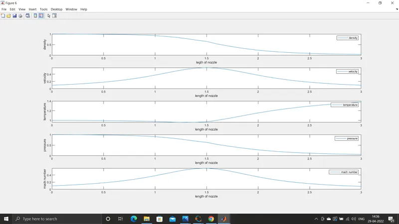
#) Plot for the conservative equations is

#) variation of the non- dimensional mass flow with time

#) Timewise variation of variable at throat-

#) Variation of normalized mass flow rate distribution for both forms-

#) The grid Independent study-

sl. No	number of grid points	density for conservative	temperature for conservative	pressure at conservative	mach number at conservative	Density at non conservative	temperature at non conservative	pressure at non conservative	Mach number
1	31	0.6504	0.840	0.546	0.981	0.638	0.836	0.534	0.999
2	93	0.6373	0.8359	0.532	1.001	0.836	0.836	0.535	1.003
3	155	0.6415	0.837	0.537	1.0034	0.634	0.850	0.528	1.019

The above solution represents the steady state solution at the throat section in the nozzle for both the cases. the deviation from the original value bis very marginal for the grid numbers of 93 and the 155 . thus increasing grid points will increase the accuracy both it will take more time.

#) conclusion-

1) the program was written for both the forms and in Matlab.

2)It can be inferred from the steady state distribution of primitive variables inside the nozzle for both the forms that there is no much difference of the values in both the form as it can be observed in the grid independent test.

3) It can be inferred from the variation of the primitive variable for both the form that the largest changes take place at the earliest time steps after 400 timesteps the value of the primitive variable reaches to the steady state.

4) it can be inferred from the comparison of the normalized mass flow rate distribution to both the form that the mass flow rate predicted by the conservation form of the equation is much more satisfactory than the non conservative form of the equation on the basis of two accounts that the conservation form is much closewr to the 0.579. On the other hand in non - conservative form some spurious oscillation can be found at the inlet and outlet of the nozzle. The conservation form of the equation is closer to the analytical mass flow rate.

5) The execution time for the conservation form of the equation is 1.361 and the non- conservative form is 2.472.

6) It can be inferred from the variation of the non- dimensional mass flow rate along the nozzle for different time steps in nonconservative form . After 50 iterations the mass flow rate has changed drastically and after 100 iterations the mass flow rate has changed after 700 iterations the solution stabilizes and after 1400 iterations the mass flow rate becomes steady and the solution has converged.