Week 2 - Flow over a Cylinder.
AIM- To simulate the laminar flow over the cylinder and simu8late the phenomena of vortex shredding and calculate the Strouhaul number of the flow. By varying the Reynold number from 10 to 10000 we can see how the drag coefficient changes due to this effect.
Theory of the flow- As flow over a cylinder is one of the basic calculations in the CFD domain and till this date, the research is going on to study the unsteady behavior caused by the flow. The flow over cylinder study is very complex and the periodic flow patterns are seen at a low Reynolds number after the critical Reynolds number the flow gets changed in the wake region and this wake formation leads to Von Karman vortices. Consider any other object compared to cylinder this point of the upstream boundary layer and other flow parameters.
Laminar region to tu8rbulent region is governed by the dimensionless number of Reynold Number. tis number is a measure of different flow criteria over the region can be calculated from density of the nflow field, flow speed , characteristic linear dimension depending upon geometry, and dynamic viscosity. As he flow in the wake region may be have the periodic motion and hence we have a certain frequency with which it resonates. If the frequency matches with the frequency of the structure with which it vibrates, hence resonance can occur. The frequency of motion can be given by another dimensionless number called the Strouhal Number can be used to determine the time step for the simulation as for the specific REYNOLDS number. The vortex-induced vibration is one of the key aspects which maybe lead to the study of vortex shedding in real-life applications such as aircraft and turbine designs. The vibration caused by the vortex phenomena due to flow dynamics is needed to study and design the axial flow turbine design phenomena.
#) Solving and modeling approach-
The main aim of the project is to study the behavior of Reynolds number on the flow over cylinder to capture the flow with every regime it is important to have more flow domain or less mesh size to capture every possible vortex in the wake region.
The problem is divided into two groups in which both the steady and the unsteady state simulation. Simulation of the varying Reynold number will be taken into consideration by maintaining fluid property constant changing the Reynolds number from 10, 100,1000,10000,100000 and accordingly the parameters are studied. The problem will start with the 2 - dimensional geometry of the flow field and the mesh is created accordingly . Firstly the mesh element size is kept at a high value for steady-state analysis since we do not have to capture what is going on between the time steps.' For the transient state analysis, we use a much finer mesh by introducing more number of elements and nodes and introducing the number of divisions around the cylinder structure and the inflation is also added to finer the mesh. The inflation layer will be added near the cylinder to capture the boundary layer detachment from the surface of cylinder. As it is to stand to perform unsteady state simulation this project will incorporate special method to solve the problem with the traditional method and non iterative time advancement(NITA) method.
The solver is much towards time marching problem with greater ease and with less number of iterations.
The boundary condition will be simple as velocity inlet and pressure outlet with symmetry wall type condition. The cylinder will also considering as well type on which coefficient of lift and drag will be calculated.
#) For steady state solver the SIMPLE algorithm is used which stands for the semi-implicit method for pressure linked equation.
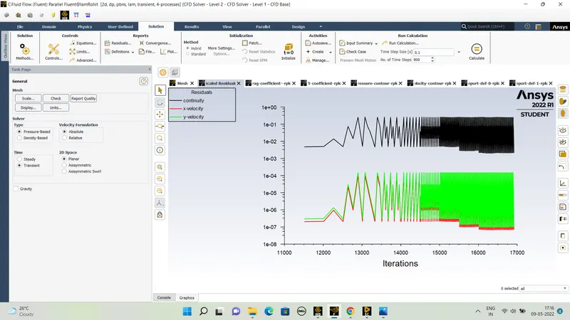
to calculate results in the neighboring volume. Unsteady state simulation is done by both the SIMPLE algorithm and the PISO algorithm also known as pressure implicit with the splitting of operators with large time steps and less computing effort. It is an extension of teh SIMPLE algorithm. To check for convergence of the solution we will create some plots that will be behind the 10 m behind the cylinder. Which would be used to plot the Strouhul number later using the FFT option in the Fluent.
The Reynolds Number of the flow is defined as the
Re =(rho*v*d)/viscosity.
rho is the density of the fluid taken as 1 kg/m^3.
v is the velocity of thye flowing fluid.
d - dimaeter of the cylinder. It is fixed by the geometry = 2 m.
viscosity is kept at the 0.05 Ns/m^2.
The meaning of the Reynolds number is the ratio of the inertial force to the viscous force which means for the laminar flow in which the Reynolds number is up to 1000 the viscous force have some effect from 1000 to Re = 5000 this is a transition region and when the Reynolds number is above 5000 the flow becomes turbulent viscous force becomes much less.
The coefficient of drag is obtained
cd = (2*Fd)/(density* velocity^2*area)
Fd - drag force
The coefficient of the lift is
cl = (2*Fl)/(density*velocity^2*area)
Fl - the lift force.
area is the frontal area.
case1) - Simulation of a flow over a cylinder with Re = 100
v = 2.5 m/sec.
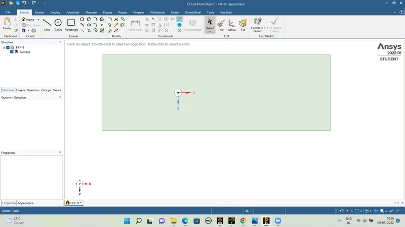
#) The geometry of the figure or the CAD model is -
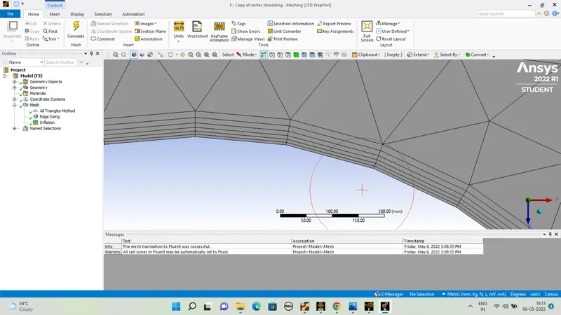
The finer that was created in the mesher in the workbench is -
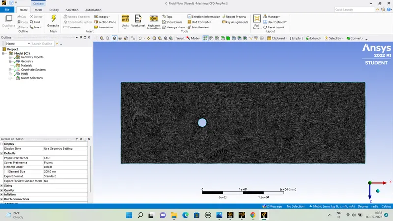
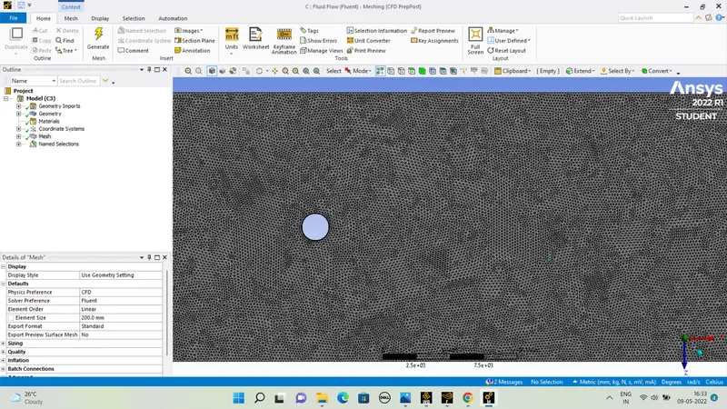
Here the all triangular method is used so that the orthogonal elements are transformed into the triangular mesh elements.
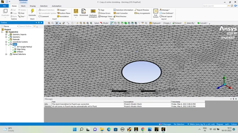
Thirdly the inflation layer is also added and 6 layers are being added with a growth factor of 1.2.
#) The mesh metrices are shown as -
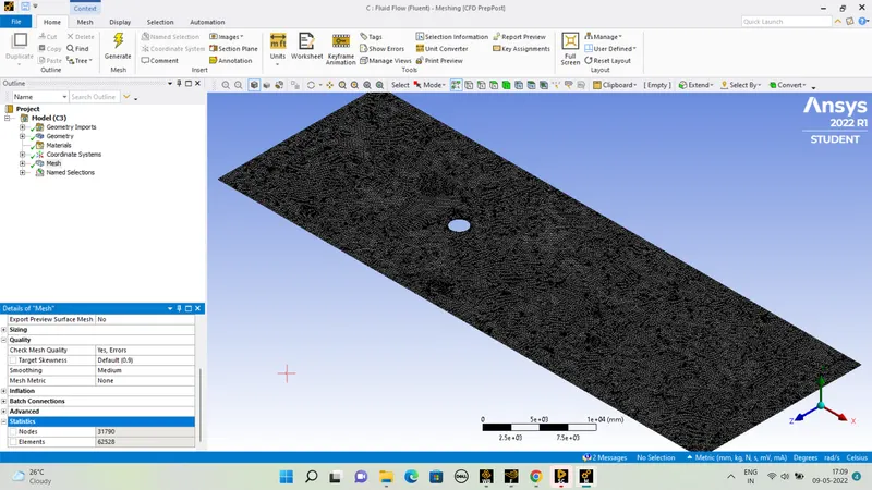
So the mesh contains more thyan 62000 elemesnts and the nodes are of more than 31000. The quality of the mesh is also shown in the quality section.
#) The different sections of the object is also needed to be named using the name selection at the edges of the sections
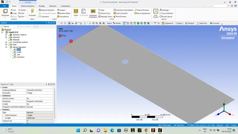
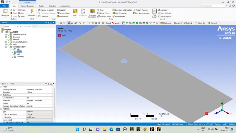
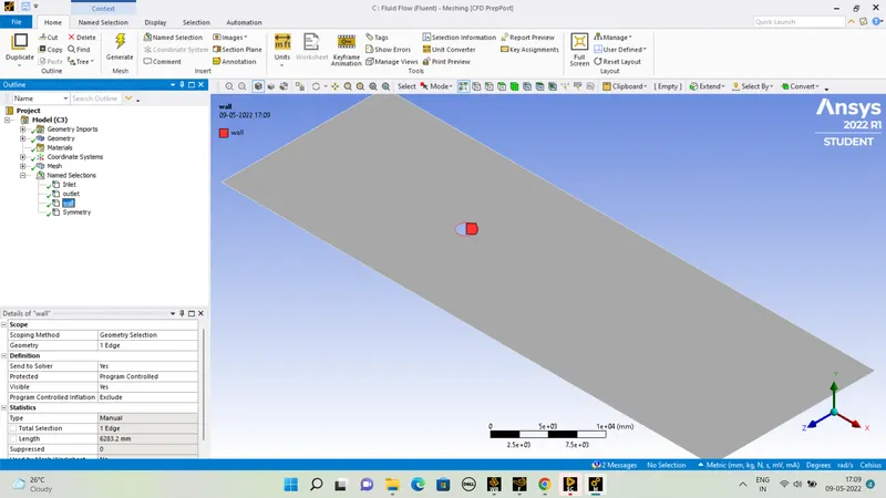
For the velocity of flow = 2.5m/sec. We have the Reynold number to be only of Re= 100
The outcomes obtained in the steady-state simulation using the SIMPLE solver -
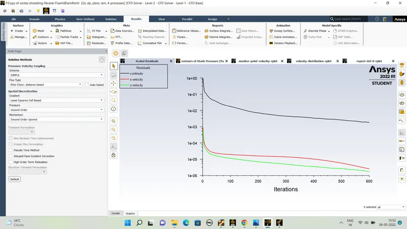
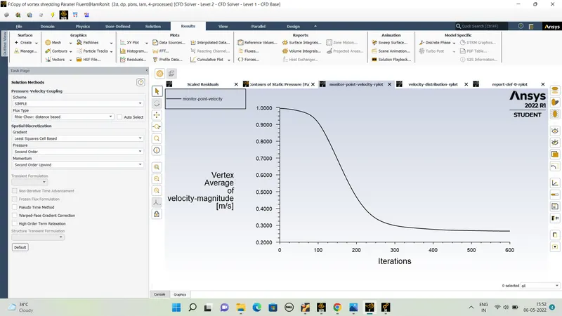
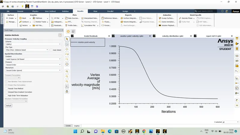
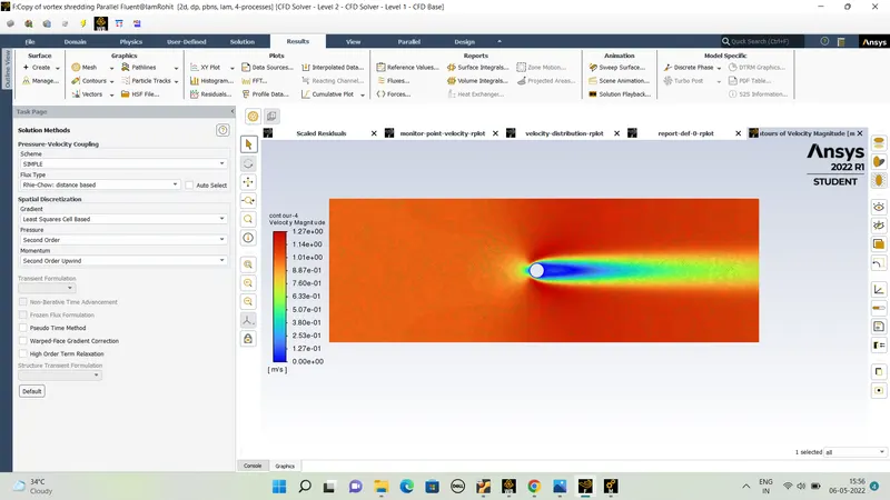
#) The transient simulation is conducted for the Re = 100 using the pressuree velocity coupling with the SIMPLE solver-
Finer mesh is used to help to capture the time-dependent variation in the quantities like the lift coefficient na the drag coefficient and the velocity contour developed and the vertex average velocity .
the results obtained are-
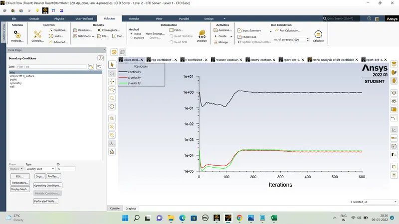
The residuals-
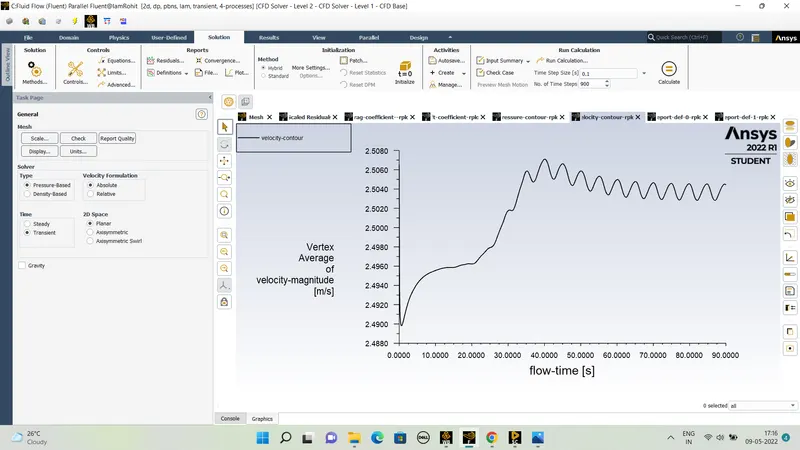
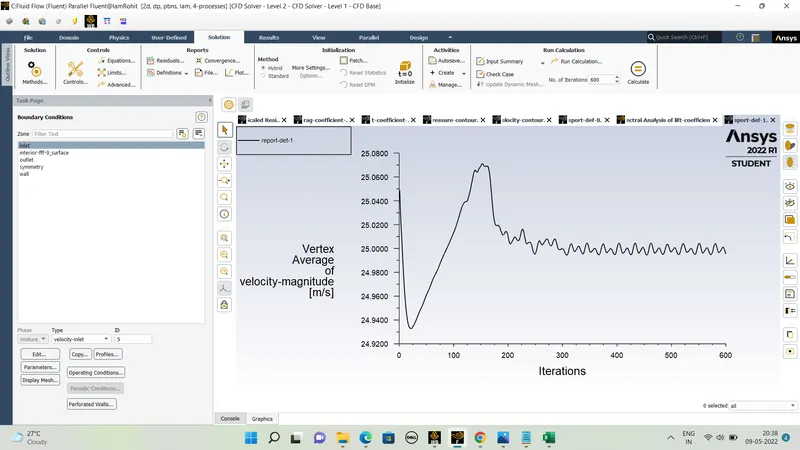
#) The vertex average of the velocity magnitudes-
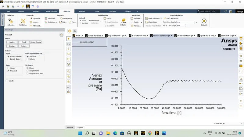
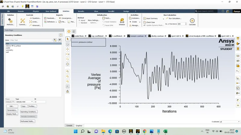
#) The Vertex average of the pressure-
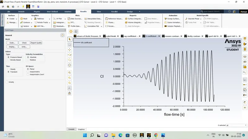
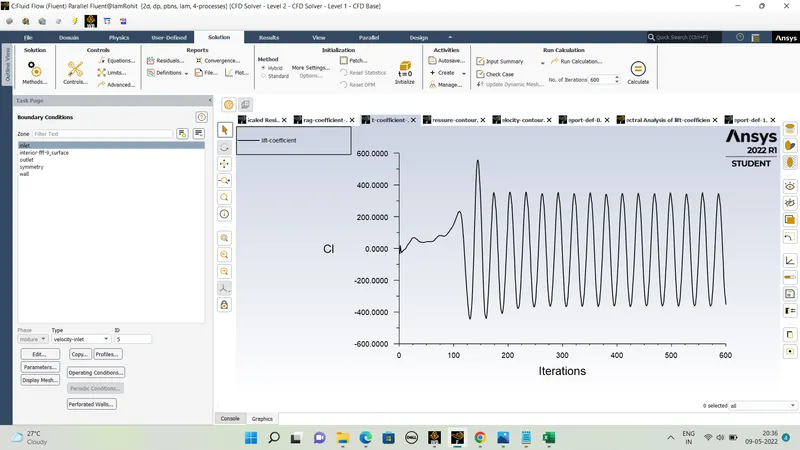
#) The lift coefficient variation with the flow time as the iteration is done for more number of iterations l9ike 900 we get cl value keeps on oscillating between a , maximum and minimum value indicating we can find the frequency of the oscillation and the subsequent Strouhal Number-
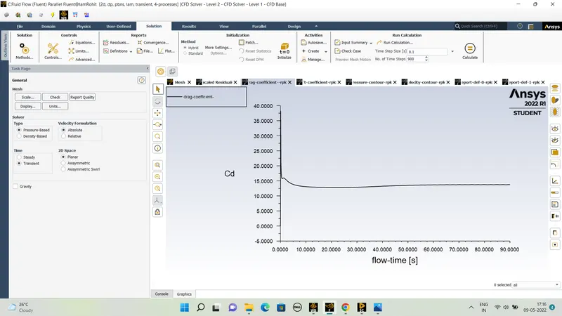
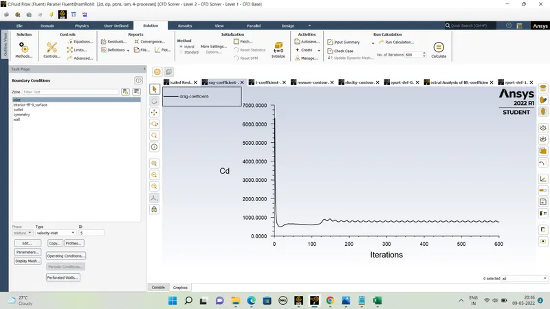
#) the drag coefficient with flow time-
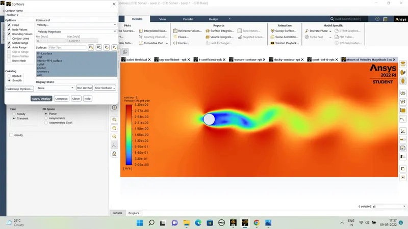
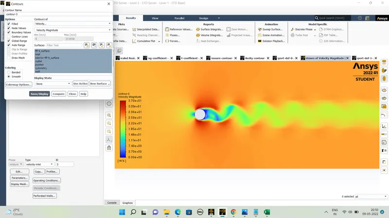
#) The velocity contour - In the Reynolds Number = 100, Where the velocity is of = 2.5m/sec, viscosity = 0.05 kg/m-s. and the characteristics length or the diameter of the sphere = 2m we are able to see the phenomena of vortex shedding
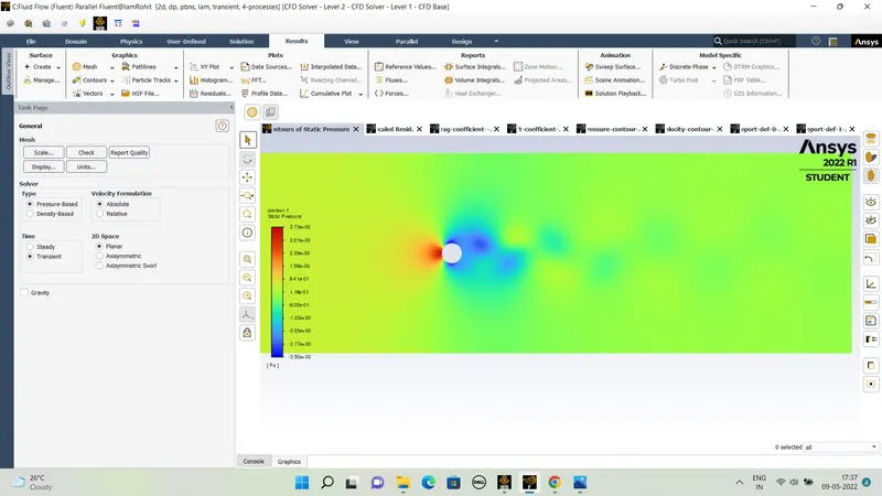
#) The pressure distribution -
#) The magnitude variatin along with the Strouhal number in the x axis-
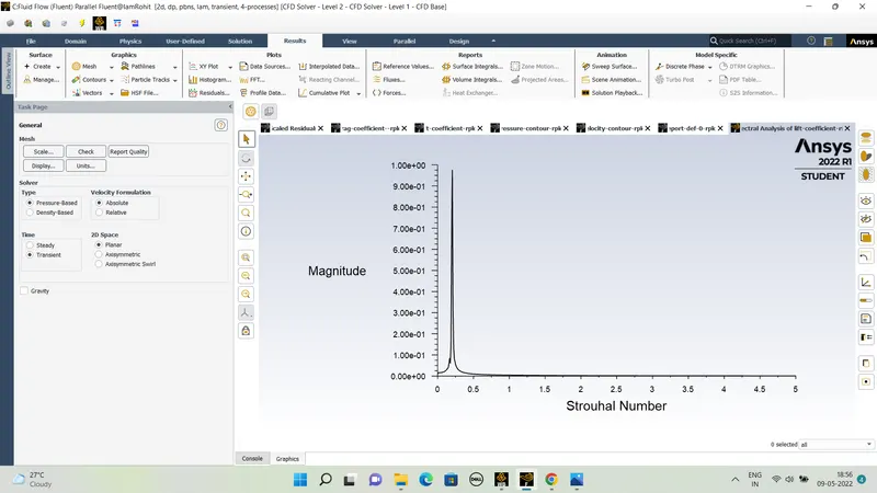
#) To calculate the Strouhal number - Strouhal numkber is a dimensionless number describing the oscillating flow over any object . For large Strohal number order of 1 viscosity dominates fluid flow resulting in a collective oscillating movement . For low Strouhal number of the order of 10^-4 and below the high speed quasi-steady state portion of the movement dominates the oscillation. Oscillation at the intermediate level Strouhal number is characterized by the buildup and rapidly subsequent shedding of vortices.
The FFT is done on the quantity of the lift coefficient (cl).
The Strohal number is given by
sr = fD/u'.
f is the frequency of vortex shedding
D is the characteristics diameter .
u' is the fluid flow velocity.
we have to the fast fourier transform also called as the FFT or the fast fourier transform-
The excel sheet data obtained of the Strouhal number and the magnitude is
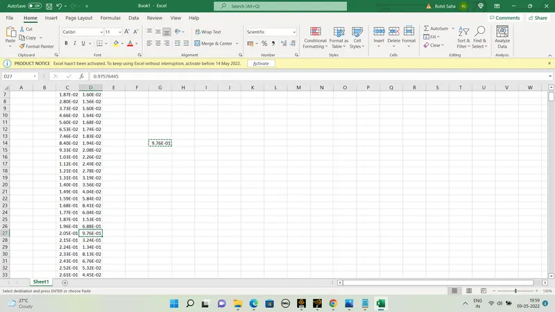
The maximum magnitude is of 9.76E-01. So the corresponding 2.05E-01 .
So , Strouhal number of the transient oscillation for Reynolds number = 100 velocity = 2.5 m/sec is equal to = 2.05E-01.
#) CASE-2 with varying Reynolds number- For the Reynolds number = 1000 so the freestream velocity v= 25 m/sec and the viscosity = 0.05 kg/m-sec.
By using the SIMPLE algorithm for the same mesh
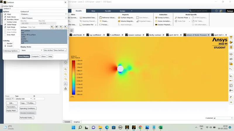
#) For Reynolds Number Re = 10000 V= 250 m/sec and keeping all other parameters same
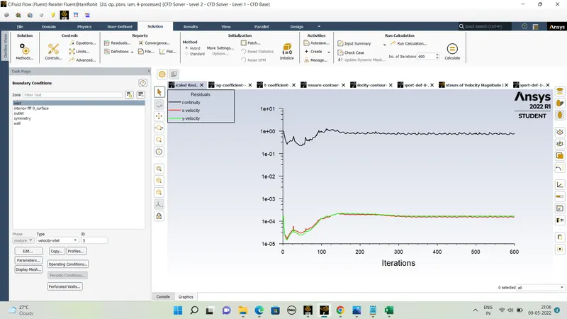
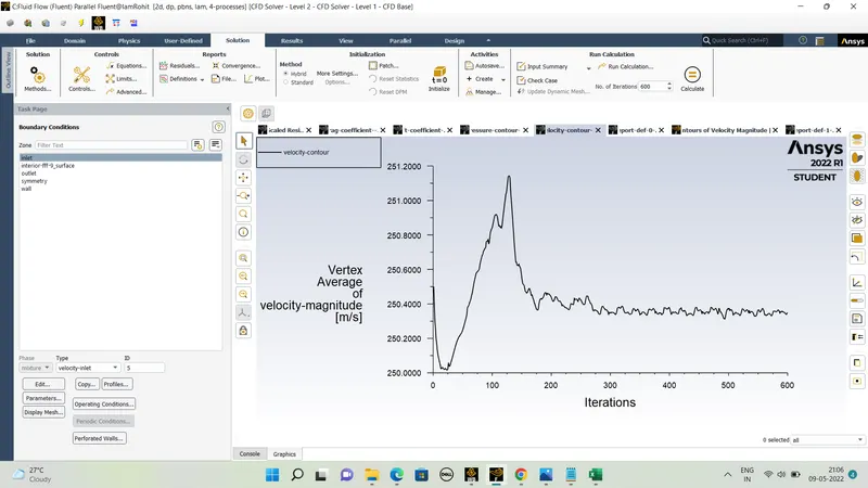
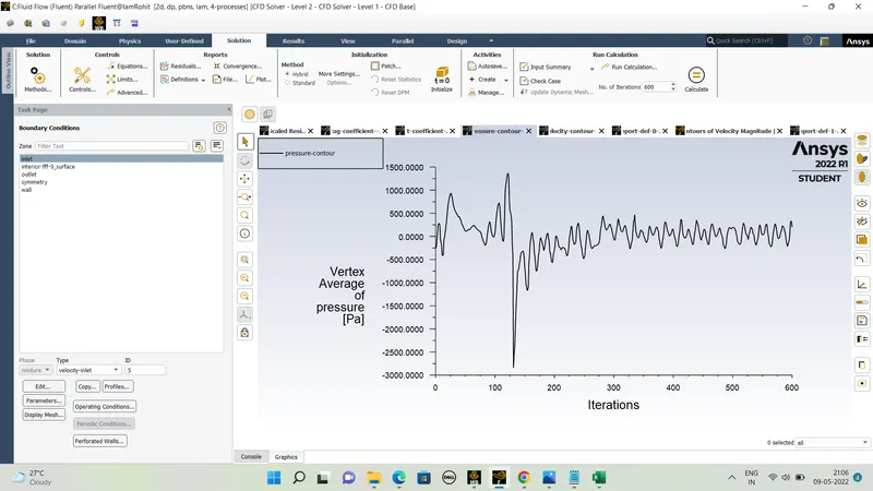
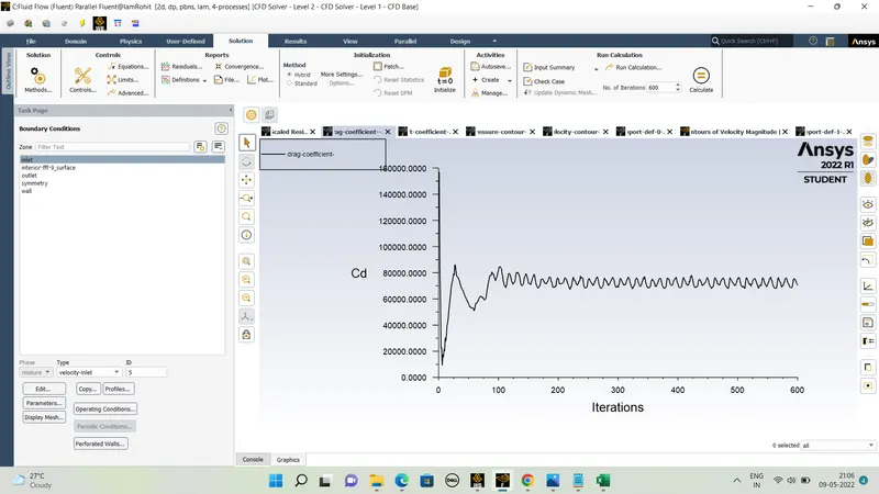
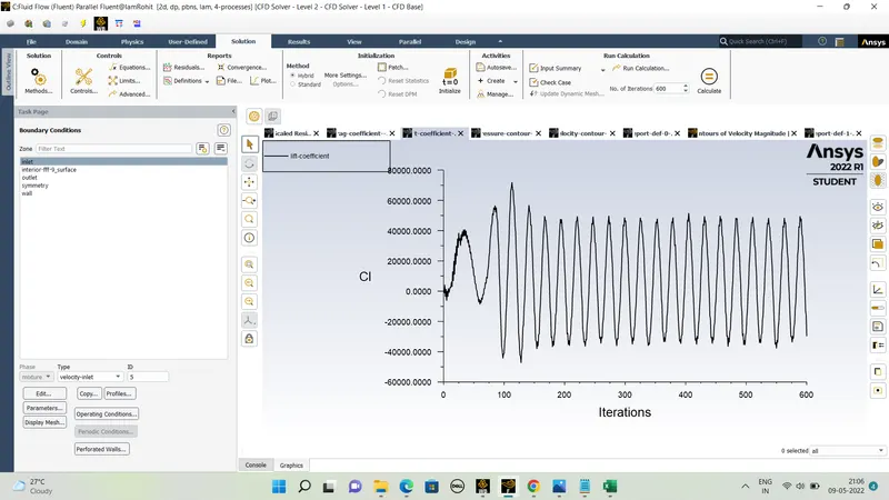
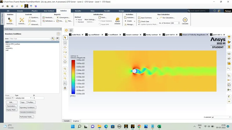
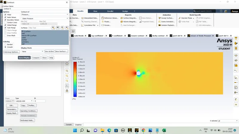
#) For Re = 100000 v= 2500 m/sec.
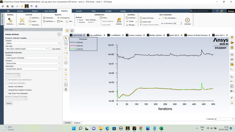
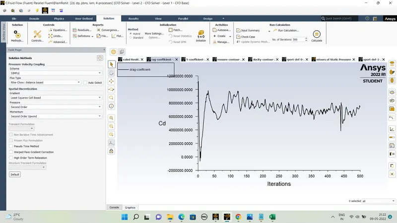
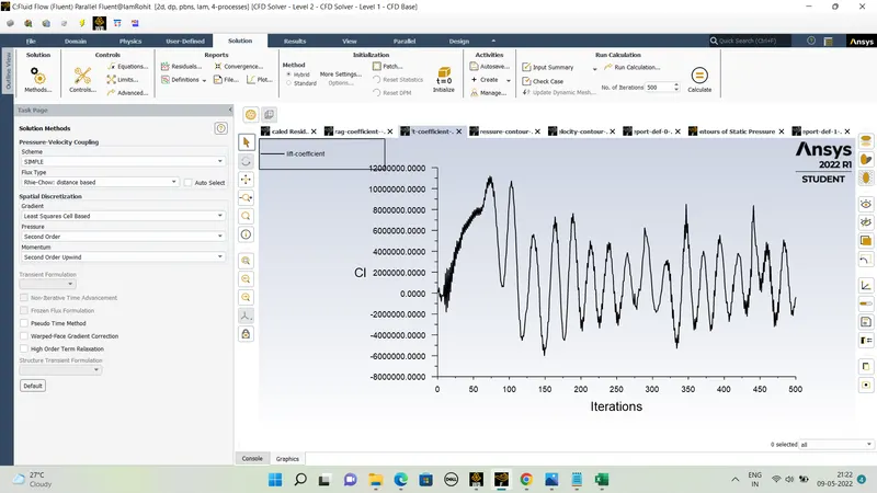
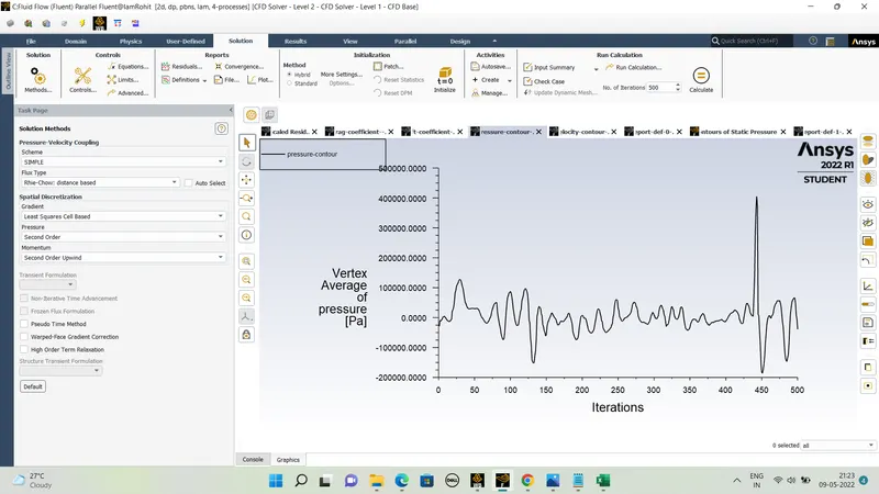
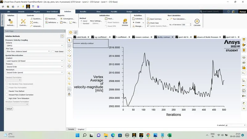
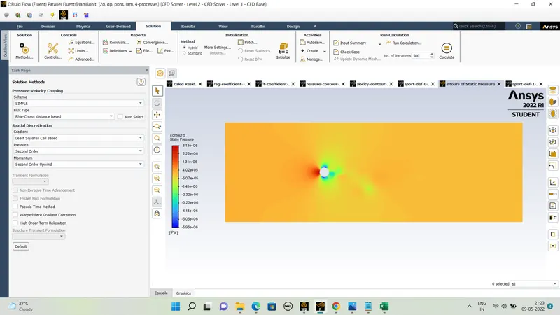
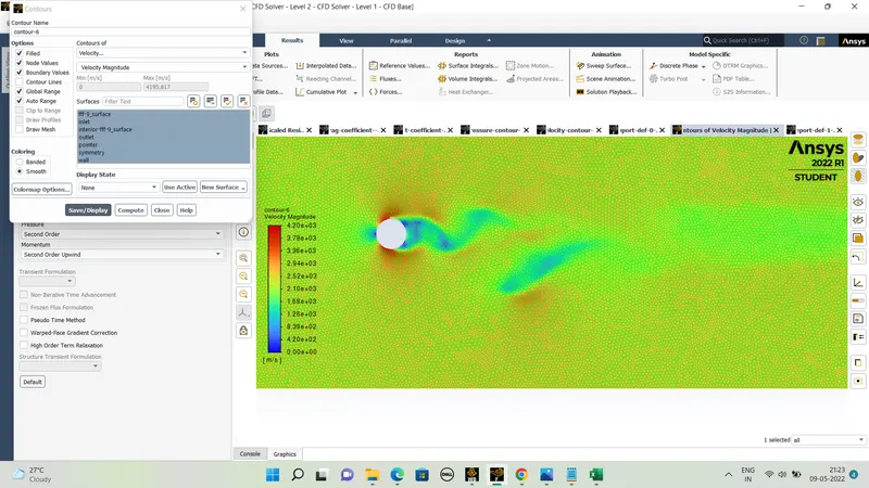
It is clear that once Reynolds number is increased beyond a critical value we can be able to see flow separation due to the boundary layer separation. Since the cl value keeps on oscillating we are taking the value of the average cl value that will be printed in the comnsole.
Effect of Reynolds Number on the drag coefficient-
#) Comparison of the lift and drag coefficient w.r,t Reynolds number-
Reynolds Number drag coefficient lift coefficient
10 3.37 0.0011
100 1.31 0.048
1000 1.08 0.048
10000 1.18 0.562
100000 0.85 0.672
#) Conclusions-
1) It is quite clear as the Reynolds number increases the coefficient of drag also decreases and vice versa happens with the lift coefficient. The data is compared with the research paper that is given for reference.
2) The phenomenon is happening because of the friction between the moving air and the surface of the cylinder. It causes the boundary layer to break down before floe separation hence we get flow separated hence amount of drag gets decreased and the lift is increased.
3) S the Reynolds number increases there is a need to keep larger domain size behind the cylinder which results in in bigger flow domain capturization.
4) For low Reynolds number vortices are a bit symmetrical but when the Reynolds number is high the vortices tend to lose their shape and become irregular inj geometry.
5) It can be seen that the steady-state simulation takes less time to converger to a physically acceptable solution and when the transient and time-dependent simulation is simulated which captures each frame at a certain time step it takes a much higher time to converge. The transient simulation captures each and every frame for the given number of time steps.