Week 5.1 - Mid term project - Solving the steady and unsteady 2D heat conduction problem
AIM- To solve a 2D heat conduction equation over a flat plate where the boundary conditions are being given. We are going to separately code for the the steady and the unsteady parts of the two-dimensional heat conduction equation.
The partial differential equation that defines the entire physics of the 2-D heat conduction equation is the steady and the unsteady problem is -
`(delu)/(delt) = alpha*((del^2u)/(delx^2)+(del^2u)/(dely^2))`. In this case we take u as the temperature = T(x,y,t).
Since it is a partial differential equation Temperature is dependent on the two spatial terms and the time also.
delT/delt represents the partial derivative of the temperature with respect to the time.
`del^2T/delx^2 represents the second-order partial derivative of the temperature w.r.t x`
del^2T/dely^2 represents the second-order derivative of the temperature w.r.t y.
The spatial derivatives were discretized by the central differencing schemes-
T(i,j) = ((deltax^2*deltay^2)/2*(deltax^2+deltay^2))*[(Ti-1,j+Ti+1,j)/deltax^2+(Ti,j-1+Ti,j+1)/deltay^2].
Code for the steady-state two - dimensional heat conduction equation-
% To write a program to do the steady state two dimensinal heat conduction
% equation over  a flat plate

clear all
close all
clc

% To write down the parameters
L = 1 ;
nx = 100 ;
ny = nx ;
x = linspace(0,L,nx) ;
dx = x(2)- x(1) ;
y = linspace(0,L,ny) ;
dy = y(2)- y(1) ;

% Guess temperature matrix
 T = 300 * ones(nx,ny) ;
 T(:,1) = 400 ;
 T(1,:) = 600 ;
 T(:,end) = 800 ;
 T(end,:) = 900 ;

 T_old = T ;
 term = (dx^2*dy^2)/(2*(dx^2+dy^2)) ;
 tol = 1e-4 ;
 error = 1 ;

 iteration_method = 1 ; % iteration_method=1-jacobi ;2-gauss siedel;3-SOR
 if iteration_method == 1 % jacobi method
     tic
     iter = 0 ;
     while(error>tol)
         for j = 2:ny-1
             for i = 2:nx-1
                 T(i,j) = term* ((T_old(i-1,j)+T_old(i+1,j))/(dx^2)+(T_old(i,j-1)+T_old(i,j+1))/(dy^2)) ;
             end
         end
         error = max(max(abs(T-T_old))) ;
         T_old = T ;
         iter = iter+1 ;
     end
     time = toc ;


 elseif  iteration_method == 2 % gauss siedel method
     tic
     iter = o ;
     while(error>tol)
         for j = 2:ny-1
             for i = 2:nx-1
            T(i,j) = term* ((T(i-1,j)+T_old(i+1,j))/(dx^2)+(T(i,j-1)+T_old(i,j+1))/(dy^2)) ;
             end
         end
         error = max(max(abs(T-T_old))) ;
         T_old = T ;
         iter = iter+1 ;
     end
     time = toc ;


 elseif iteration_method == 3 % Successive over relaxation
     omega = 1.8 ;
     tic
     iter = 0 ;
     while(error>tol)
         for j = 2:ny-1
             for i = 2:nx -1

                 T(i,j) = term*((T(i-1,j)+T_old(i+1,j))/dx^2+(T(i,j+1)+T_old(i,j-1))/(dy^2)) ;
                 T(i,j) = T_old(i,j)*(1-omega)*(T(i,j)) ;
             end
         end
         error = max(max(abs(T-T_old))) ;
         T_old = T ;
         iter= iter+1 ;
     end
      time = toc ;

      end


      % plotting the contour on x and the y axis
      [c,h] = contourf(x,y,T) ;
      clabel(c,h)
      colorbar
      colormap(jet)
      ax = gca ;
      ax.YDir = 'reverse' ;

      xlabel('xaxis')
      ylabel('y-axis')
      title({'steady state temp profile';['Iteration Method=',num2str(iteration_method)];['no of iterations=',num2str(iter)];['simulation time=',num2str(time),'s']})
      grid on
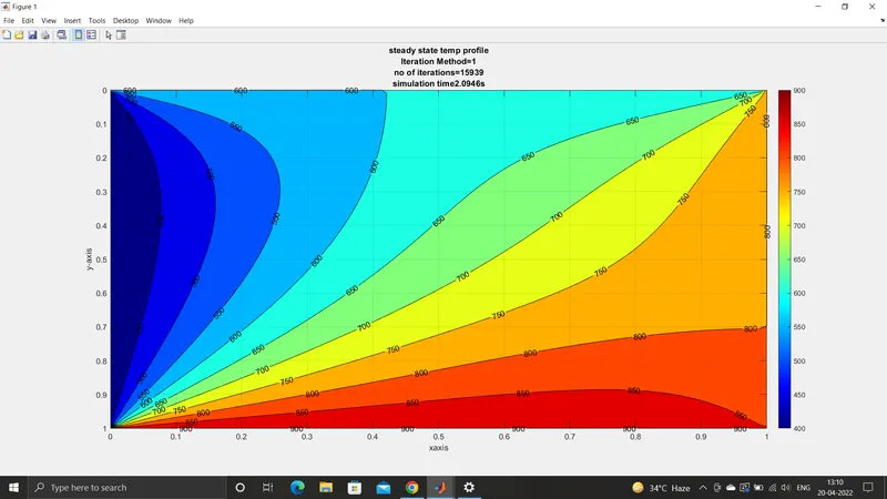
Outcome- plot of project-
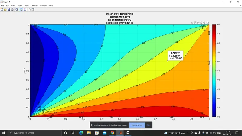
2) The iteration contour plot for the second iteration-
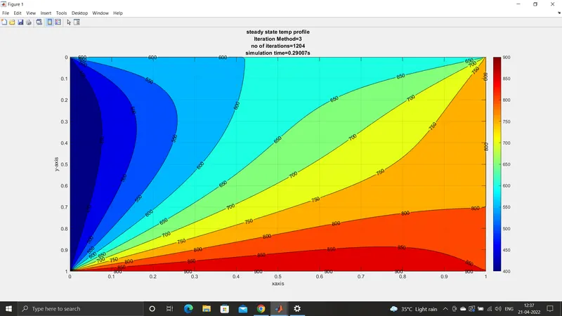
3) The contour plot of steady state temperature profile using the successive over relaxation solver-
#) Explanation of the code-
1) First the parameters of the problem to be solved like the domain length is needed and the mesh size or the step size is needed to be defined.
2) The boundary condition temperatures given in the problem is also defined. Using the command used in the matrix format.
like the T(:,1) which represents the temperature in the first column. The term which is coded separately will be used in the main formula as the word of the term.
3) Then the iteration method is used to use each of the three solvers separately in the solution of the discretized algebraic equations. The first solver used in this process is the Jacobi method to solve we are using the conditional statement while since the iterations will only run when the error is greater than the tolerance limit. Once the error drops to a low value after performing many iterations then the solution is said to be converged. Since the domain is created using the nx and the ny command. We are using the two for loops to continue the iteration for the entire length of nx and ny and removing the endpoints or the boundary points are not included in the iteration because the value at those points is already known.
4) The same procedure is followed for the other two solvers which means we have to give the same error and tolerance condition and the two for loop is used to run the iteration for the entire domain to get the temperature at every nodal points.
5) Then using the contourf command is used to create the visual of the temperature distribution.
6) The title command is used to show on the picture the type of solver used, the number of iterations done untill convergence is achieved and the time taken for the entire iteration is also shown on the picture of the temperature distribution profile as shown above.
2) The code for the transient or time-dependent pde is taken into consideration- The explicit Scheme of the time-dependent equation-
% equation
clear all
close all
clc

% parameters
L =1 ;
nx = 100 ;
ny = nx ;
dt = 0.14 ;   % time steps
t = 500 ;
nt = t/dt ;
alpha = 1.75e-4 ;
x = linspace(0,L,nx) ;
dx= x(2)-x(1) ;

y = linspace(0,L,ny) ;
dy = y(2)-y(1) ;
CFL = alpha*dt*((1/dx^2)+(1/dy^2)) ;

% Guess temperature matrix
T = 300*ones(ny,nx) ;
T(:,1) = 400 ;
T(1,:) = 600 ;
T(:,end) = 800 ;
T(end,:) = 900 ;
T_old =  T ;
k1 = alpha*(dt/dx^2) ;
k2 = alpha*(dt/dy^2) ;

iter = 0 ;
tic
% time loop
for k = 1:nt
% space loop
for j = 2:ny-1
    % x- space loop
    for i = 2:nx-1

        H= (T_old(i-1,j)-2*T_old(i,j)+T_old(i+1,j)) ;
        V= (T_old(i,j-1)-2*T_old(i,j)+T_old(i,j+1));
        T(i,j) = T_old(i,j)+(H*k1)+(V*k2) ;
    end
end
T_old = T ;
iter= iter+1 ;
end
time = toc ;


      % plotting the contour on x and the y axis
      [c,h] = contourf(x,y,T) ;
      clabel(c,h)
      colorbar
      colormap(jet)
      ax = gca ;
      ax.YDir = 'reverse' ;

      xlabel('xaxis')
      ylabel('y-axis')
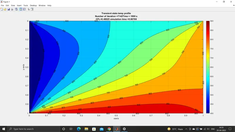
      title({'Transient state temp profile';['Number of iteration =',num2str(iter),'Time = ',num2str(t),' s'];['CFL=',num2str(CFL),' simulation time =',num2str(time)]})
      grid on
#) In converting the time-dependent terms into the algebraic equations or we are using the forward differencing to the time derivative terms, and we would be using the central differencing scheme to the spatial derivatives we obtain the following equation-
T(i,j)^n+1 = T(i,j)^n+ alphadeltat/deltax^2(T(i-1,j)-2*Ti,j+T(i+1,j)^n+alphadeltat/deltay^2(T(i,j-1)-2*T(i,j)+T(i,j+1))^n.
Since we are solving the equation explicitly so in the RHS we only need the value of the temperature of the previous node that is represented by n and in the LHS we are able to get the value of temperature at the n+1 node. So we are actually obtaining the linear algebraic equations which are not coupled like those that appear in the implicit way of solving.
#) In the code we are coding the variables that is the k1 and the k2 which is the k1 = alpha*(dt/dx^2)
and k2 = alpha*(dt/dy^2).
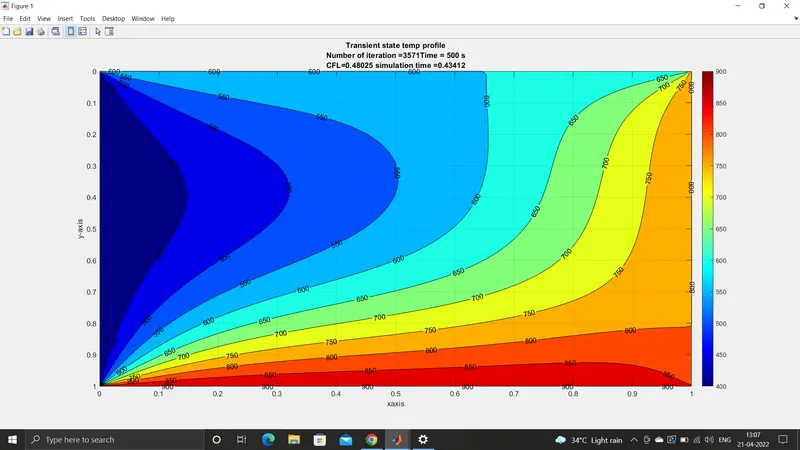
Outcome of the project or the temperature distribution profile-
1) When the time given to study the temperature distribution is t = 500 seconds
2) when the time given is for t = 1000 seconds
3) Code for the Implicit scheme to solve the two-dimensional transient heat conduction equation-
% To write a code to solve the two dimensional heat conduction equation by
% implicit equation solving

clear all
close all
clc

% parameters
L = 1;
nx = 50 ;
ny = nx ;
dt = 10 ;
t = 1000 ;
nt = t/dt ;
alpha = 1.75e-4 ;
x = linspace(0,L,nx) ;
dx = x(2)-x(1) ;
y = linspace(0,L,ny) ;
dy = y(2)-y(1) ;

CFL = alpha*dt*((1/dx^2)+(1/dy^2)) ;

% Guess temperature matrix
T = 300*ones(ny,nx) ;
T(:,1) = 400 ;
T(1,:) = 900 ;
T(:,end) = 800 ;
T(end,:) = 600 ;
T_old =  T ;
T_prev = T ;
k1 = alpha*(dt/dx^2) ;
k2 = alpha*(dt/dy^2) ;

tol = 1e-4 ;

iteration_method = 2 ; % Iteration_method = 1-Jacobi ; 2-Gauss siedel ;3-SOR

% Jacobi method
if iteration_method ==1
    tic
    iter = 1 ;
    for k = 1:nt
        error = 1;
        while error>tol
            for j = 2:ny-1
                for i = 2:nx-1

                    term1 = 1/(1+2*k1+2*k2) ;
                    term2 = k1*term1 ;
                    term3 = k2*term1 ;

                    H =(T_old(i-1,j)+T_old(i+1,j)) ;
                    V = (T_old(i,j-1)+T_old(i,j+1)) ;
                    T(i,j) = (T_prev(i,j)*term1)+(H*term2)+(V*term3) ;
                end
            end
            error =   max(max(abs(T-T_old))) ;
            T_old = T ;
            iter = iter+1 ;
        end
        T_prev = T ;
    end
    time = toc ;


    % Gauss siedel method

elseif iteration_method==2

    tic
    iter =1 ;
    for k = 1:nt
        error = 1;
        while error>tol
            for j = 2:ny-1
            for i = 2:nx-1

                term1 = 1/(1+2*k1+2*k2) ;
                term2 = k1*term1 ;
                term3 = k2*term1 ;

                H =(T(i-1,j)+T_old(i+1,j)) ;
                V = (T(i,j-1)+T_old(i,j+1)) ;
                T(i,j) = (T_prev(i,j)*term1)+(H*term2)+(V*term3) ;
            end
        end
        error =   max(max(abs(T-T_old))) ;
        T_old = T ;
        iter = iter+1 ;
    end
    T_prev = T ;
end
time = toc ;


% SOR method

elseif  iteration_method == 3
    omega = 1.1 ;
    tic
    iter = 1;
    for k = 1:nt
        error = 1 ;
        while error>tol
            for j = 2:ny-1
                for i = 2:nx-1

                    term1 = 1/(1+2*k1+2*k2) ;
                    term2 = k1*term1 ;
                    term3 = k2*term1 ;
                    H =(T(i-1,j)+T_old(i+1,j)) ;
                    V = (T(i,j-1)+T_old(i,j+1)) ;
                    T(i,j) = (T_prev(i,j)*term1)+(H*term2)+(V*term3) ;
                    T(i,j)= T_old(i,j)*(1-omega)+omega*T(i,j) ;
                end
            end
            error = max(max(abs(T-T_old))) ;
            T_old = T ;
            iter = iter+1 ;
        end
        T_prev = T ;
    end


    time = toc ;
end


    % plotting the contour on x and the y axis
    [c,h] = contourf(x,y,T) ;
    clabel(c,h)
    colorbar
    colormap(jet)
    ax = gca ;
    ax.YDir = 'reverse' ;

    xlabel('xaxis')
    ylabel('y-axis')
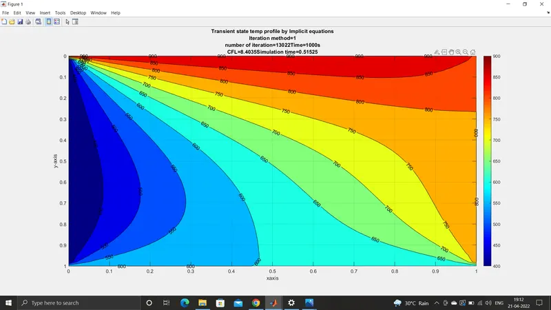
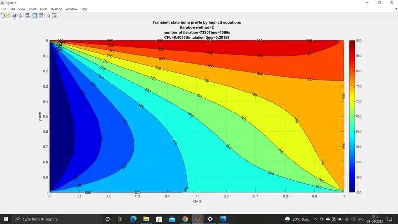
    title({'Transient state temp profile by Implicit equations';['Iteration method=',num2str(iteration_method)];['number of iteration=',num2str(iter),'Time=',num2str(t),'s'];['CFL=',num2str(CFL),'Simulation time=',num2str(time)]})
    grid on
#)The outcomes of the code in three different solvers in using the Implicit scheme-
Formula for the implicit scheme =
T(i,j)^(n+1) = T(i,j)^n + alphadeltat*[(T(i-1,j)-2*T(i,j)+T(i+1,j))/deltax^2+(T(i,j-1)-2*T(i,j)+T(i,j+1))/deltay^2)]^(n+1)
Here we have the new term or the (n+1) term in both the LHS and the RHS , it gives coupled equation which is solved in every step.
1) For the first solver using Jacobi method-
2) Using the Gauss siedel method-
3) Using the SOR iterative solver-
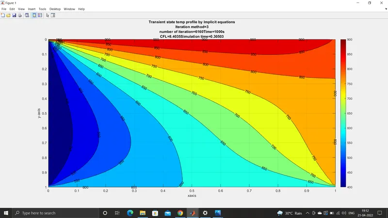
Conclusion- The two-dimensional steady and unsteady heat conduction equation was solved using both the explicit and the implicit schemes by using the iterative solvers which means we can conclude that by using an advanced solver like the successive over-relaxation we can reduce the numbers of iterations required. So the order of the number of iterations required reduces from Jacobi to Gauss-Siedel and least for the Successive over relaxation.