Week 3 - Solving second order ODEs

AIM- To write down a code in Matlab to simulate the way the pendulum oscillates.Solving the ordinary differential equation. Which would yield the result of the motion of the ball of the pendulum. Finally to create one animation of the motion so that the motion can be visualized.

Explanation- 1)ODES are the ordinary differential equations that are very extensively used in physics and engineering to describe physical phenomena. Matlab has a very special inbuilt solver to solve the odes which are called the ode45 which solves the ode once it is coded in a proper way considering the functions which are to be coded in a different window.

2)Matlab has one inbuilt solver called the ode45 it is a versatile solver it involves solving a standard second-order ODE with constant coefficients with initial conditions and non-homogenous.

3)A numerical ODE solver is used as the main tool to solve the odes. The Matlab function ode45 will be used. The important thing to remember is that ode45 can only solve the first-order ode. Therefore to solve the ode the ode needs to be first converted to the first order ode to us ethe ode45 solver.

4) Syntax for the ode45 -[t,y]= ode45(odefun,tspan, y0) . initially, the ode function is described which is separately coded as a function in a separate window. The main function is called inside the ode45 by the same name in which the function is saved in the same place. tspan is the entire time limit in which the integration is needed to be done and y0 is the initial condition of the problem.

Matlab code of the problem-

% The program to solve the two dimensional ODE of the pendulum
% To create one animation of the motion of the pendulum
clear all
close all
clc

% Inputs of the problems. The dimensions of the pendulum
% length of the chord in m
l = 1 ;
% Damping coefficient
b= 0.05 ;
% accelaration due to gravity (m/s^2)
g= 9.81 ;
% mass of the ball kg
m= 1 ;
% Initial conditions
theta_0 = [0;3] ;
t_span = linspace(0,20,200) ;
% solve ode the results contain two variables velocity and displacement
[t, results] = ode45(@(t, theta) ode_func(t,theta,b,g,l,m), t_span,theta_0);

% plotting the graph og the velocity and displacement w.r.t time
plot(t,results(:,1)) ;
hold on
plot(t,results(:,2)) ;
ylabel('plot') 
xlabel('Time in seconds')

% Iteration using for loop to create animation of simple pendulum
ct=1 ;
theta_1 = results(:,1) ;
for i= 1: length(results(:,1)) 
    % Initial co-ordinates
    x_start = 0 ;
    y_start = 0 ;
    THETA = theta_1(i) ;
    % Final co-ordinates
    x_end = l * sind(THETA) ;
    y_end = - l*cosd(THETA) ;
    
    % Plotting for animation
    figure(2) 
    % Base of pendulum
    plot([-1,1],[0,0],'linewidth',4,'Color','r' ) ;
    hold on

    % string of pendulum
    line([x_start x_end],[y_start y_end],'linewidth',6,'color' ,'b') ;
    hold on
    % bob of pendulum 
    plot(x_end,y_end,'marker','o','markersize',28 ,'markerfacecolor','r') ;
    axis([-2 2 -2 2]) ;
    hold off
    M(ct) = getframe(gcf)
    ct= ct+1 ;
end
% creating movie from captured frmae

videofile = VideoWriter("pendulum.avi",'Uncompressed AVI') ;
open(videofile)
writeVideo(videofile,M)
close(videofile) ;

Explanation- 1) In the first part the code is written to include all the constants parameters like the damping coefficient(b= 0.05), length of string mass of the bob .

2) In the second part the initial conditions like the initial displacement=0 m and the initial angular velocity= 3 rad/ sec.

3) The time period for which the motion is simulated is of 20 seconds and it is divided into 200 divisions by linspace command.

4) The solution to the ode is obtained in a two-dimensional array of [t,results]. In the result, it has the result of displacement and velocity. The ode45 solver is used inside it a coded function is given which has two variables time and displacement and time span of integration is given and the initial condition.

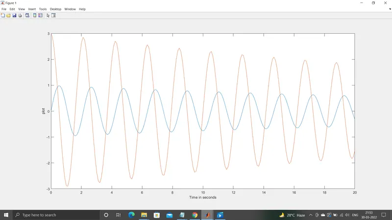
5) Plot command is used to plot the velocity and displacement by splitting into two different columns.

6) The animation is to be created by using the for loop command. we have to split down the velocity and displacement. To create the animation we use angular displacement . The value of theta_1(i) is stored in THETA.

7) The initial and final coordinates were defined by using cosd and sind of THETA. Base of the pendulum is also created and the bob of the pendulum is created by use of marker , markersize and markerfacecolor commands.

8) Axis of the figure is given for the plot.

9) To create the different figure arrays the command M(ct) = getframe(ct) is created and in200 different frames are created.

10) The video file is created by video writer command. The file is stored in the uncompressed AVI format.

Result- This is the plot of velocity and displacement plot W.r.t to time.

1)

2)Animation of the pendulum -

You tube link- https://youtu.be/J7EExL0twDs

google drive link-https://drive.google.com/file/d/1tpHKPgvUTfL31NEogt5dXrJ0A2nzsh4H/view?usp=sharing

#) Probelms faced in the project-

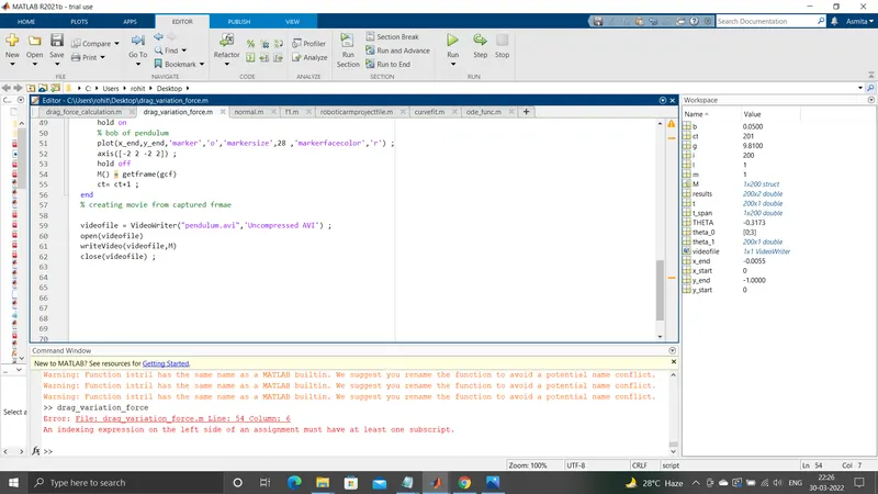
1) Problem faced during animation crearion in the M forgot to give the counter . So movie was not created.

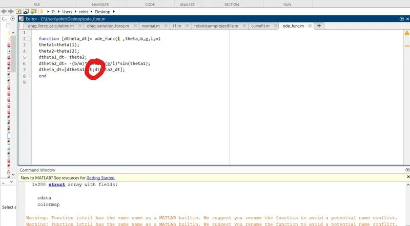
2) In the function window in the matrix we have to use the semicolon to create the coumn matrix. otherwise the main code will not be executed.

3) In the plot command proper dimenswion or co-ordinate was not used so the pendulum was not correct.

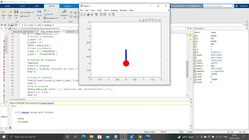
4)Previously the x_ start and x_end were not defined properly so the pendulum was upside down . The actual thing was not represented. Later the y_end sign was changed to make it the straight way.

5) Inside the for loop I forgot to denote the THETA to be equal to the loop counter so THETA= theta1(i).

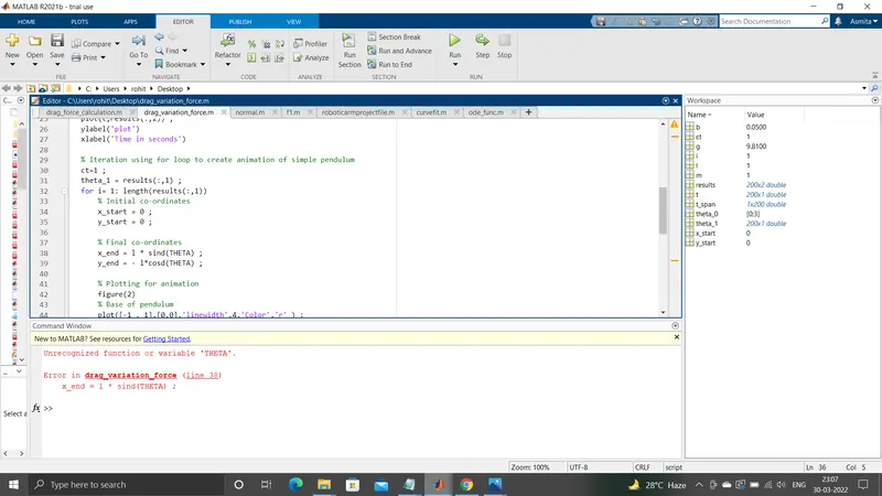
The loop counter variable should be equated to a static variable THETA . so that at each value one picture is to be created.

Conclusion- The transient or time-dependent oscillation or simple harmonic motion of the pendulum is animated, and a plot of the velocity and displacement is done with respect to time.