Simulating Mixing Tee in Ansys Fluent.
Aim: To set up steady-state simulations of mixing-tee in ANSYS-Fluent and compare the mixing effectiveness in different cases.
Objectives: To set up steady-state simulations for the following cases:
- Short length mixing tee with 36-degree Celsius inlet velocity at 3m/s and momentum ratios for the other inlet is 2 and 4 with 19-degree Celsius.
- Long length mixing tee with 36-degree Celsius inlet velocity at 3m/s and momentum ratios for the other inlet is 2 and 4 with 19-degree Celsius.
- To use the k-epsilon and k-omega SST model for the short-length mixing tee case and give a justification for using a model for the long-length mixing tee case.
- Perform the grid independence test for any one of the cases.
- Generate contour plots for velocity and temperature on the cut planes along and across the pipes.
- Generate line plots for velocity and temperature along the length of the pipe.
The Mixing Tee phenomenon has its importance for turbulent and thermal mixing and consequently for thermal striping and thermal fatigue problems in nuclear power plants. The following are the isometric views of the geometry profiles taken for our test cases:
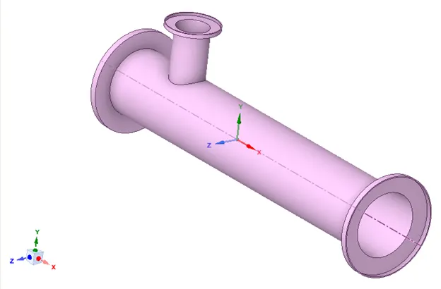
- Mixing Tee short profile.
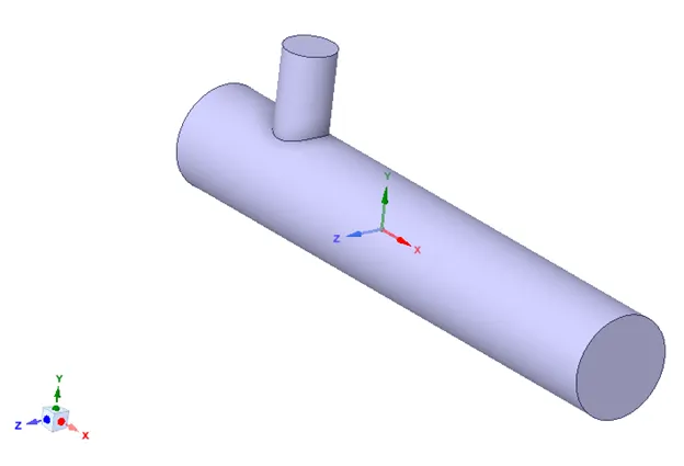
2.Mixing Tee short fluid domain.
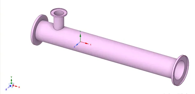
3.Mixing Tee long profile.
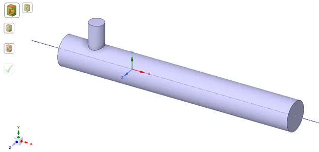
4.Mixing Tee long fluid profile.
In all our cases, the following are the solution conditions used:
- The simulation type is Steady-State simulation.
- The solver type is Pressure based.
- The Velocity Formulation is Absolute.
- The Energy Equation is turned on to set the thermal initial conditions.
- The turbulent models used are k-epsilon and k-omega and the usage cases are mentioned.
- The inlet boundary conditions at the two inlet faces are velocity inlets with an appropriate initial velocity and temperature values.
- The outlet boundary condition at the outlet face is the pressure outlet.
- The rest of the enclosing of the fluid domain is set as a stationary wall boundary condition with the no-slip condition.
Case 1: Short Mixing Tee with momentum ratio 2:
The 1st setup is by using the default mesh. The mesh quality and statistics are as follows:
|
Element sizing (By default) |
Number of nodes |
Number of elements |
|
0.010219m |
2837 |
12760 |
The views for the mesh are as follows:
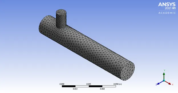
Above is the isometric view of the mesh.
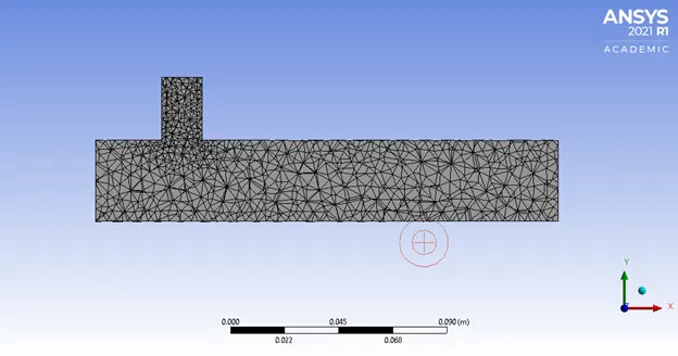
Above is the section plane of the mesh.
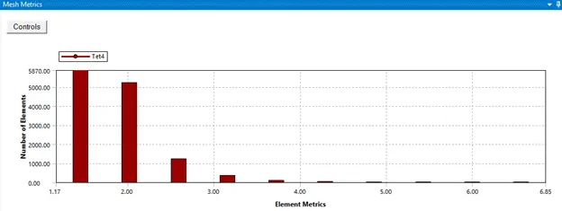
The element quality metrics are as shown below:
The initial velocity and temperature conditions are as follows:
- The velocity at the inlet in the x-direction is 3 m/s and the initial temperature is 36 degrees Celsius.
- The velocity at the inlet in the y-direction is 6 m/s and the initial temperature is 19 degrees Celsius.
The solution was run, and it achieved convergence at 230 iterations. And the following are the different plots obtained in fluent.
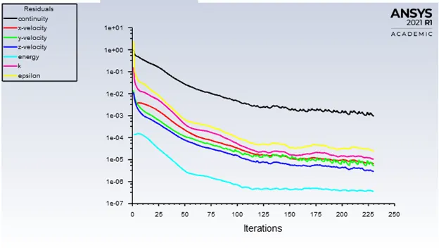
Above is the plot showing the residuals over the iterations.
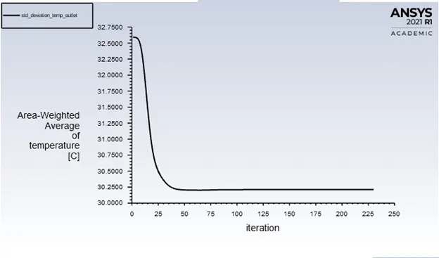
The above plot shows the standard deviation of the area-weighted average of the temperature at the outlet face over the iterations.
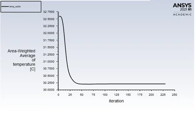
The above plot shows the area-weighted average value of the temperature at the outlet face over the iterations.
Following are the plots and results of the test case:
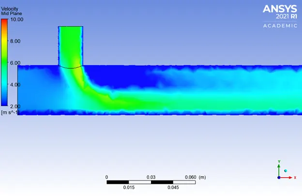
The above plot is the velocity contour plot at the mid-plane.
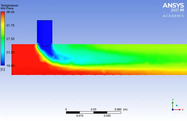
The above plot is the temperature contour plot at the midplane.
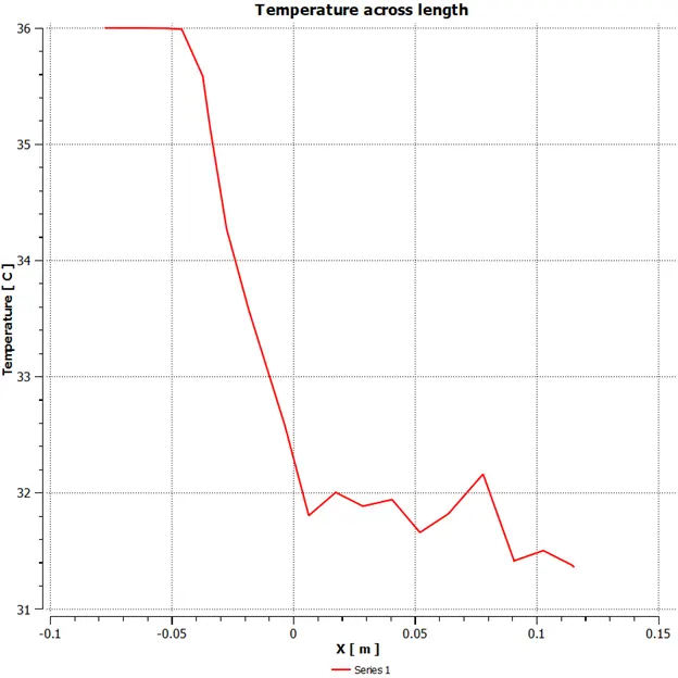
The above plot is the temperature line plot across the length of the pipe.
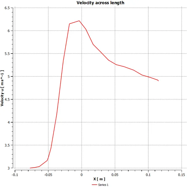
The above plot is the velocity line plot across the length of the pipe.
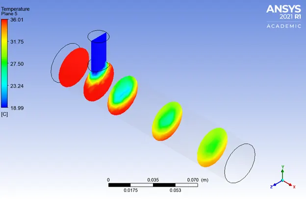
The above plot is the temperature contour plot at different cross-sections of the pipe.
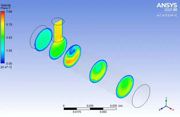
The above plot is the temperature contour plot at different cross-sections of the pipe.
The area-weighted average at the outlet face after the convergence was achieved was 30.21 degree Celsius with a standard deviation of 1.62 degree Celsius.
Case 2: Short Mixing Tee with momentum ratio 2 with a higher mesh quality:
The mesh quality and statistics are as follows:
|
Element sizing (By default) |
Number of nodes |
Number of elements |
|
0.0015m |
82747 |
455917 |
The views for the mesh are as follows:
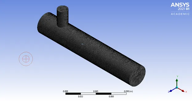
Above is the isometric view of the mesh.
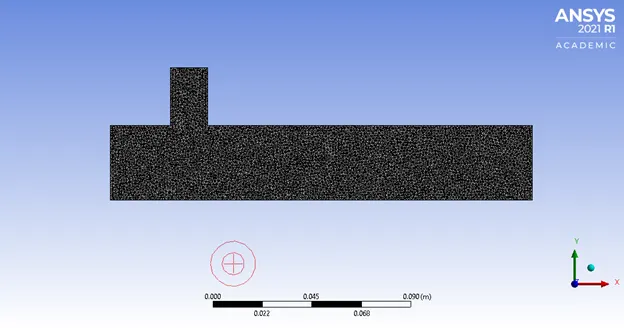
Above is the section plane of the mesh.
The element quality metrics are as shown below:
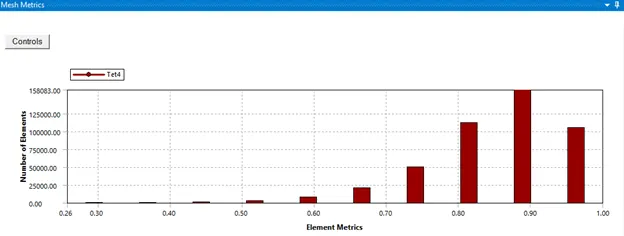
The initial velocity and temperature conditions are as follows:
- The velocity at the inlet in the x-direction is 3 m/s and the initial temperature is 36 degrees Celsius.
- The velocity at the inlet in the y-direction is 6 m/s and the initial temperature is 19 degrees Celsius.
The solution was run, and it achieved convergence at 131 iterations. And the following are the different plots obtained in fluent.
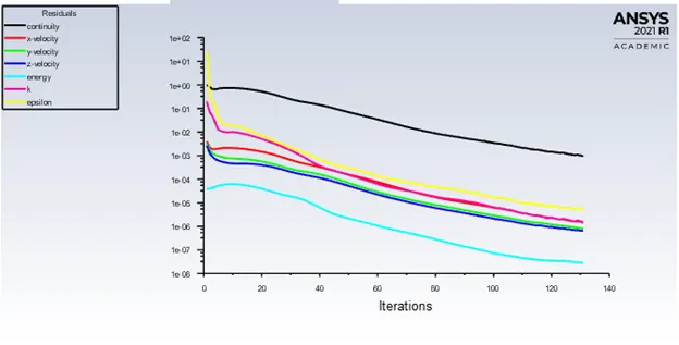
The above is the plot showing the residuals over the iterations.
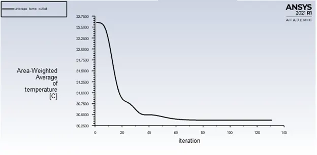
The above plot shows the area-weighted average value of the temperature at the outlet face over the iterations.
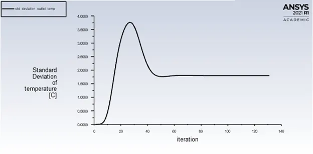
The above plot shows the area-weighted average value of the temperature at the outlet face over the iterations.
Following are the plots and results of the test case:
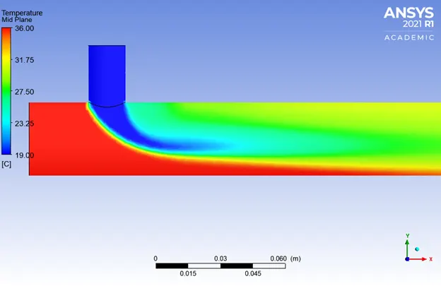
The above plot is the temperature contour plot at the mid-plane.
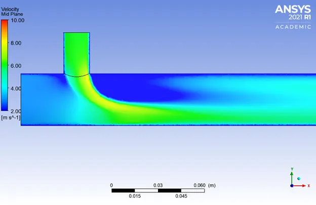
The above plot is the velocity contour plot at the midplane.
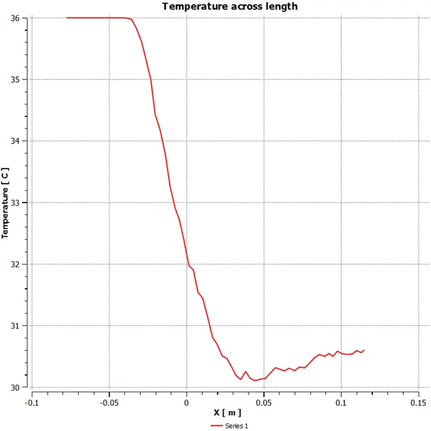
The above plot is the temperature line plot across the length of the pipe.
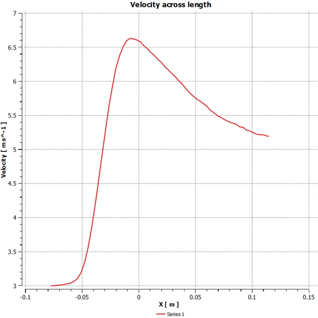
The above plot is the velocity line plot across the length of the pipe.
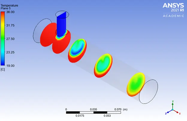
The above plot is the temperature contour plot at different cross-sections of the pipe.
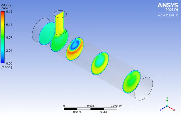
The above plot is the velocity contour plot at different cross-sections of the pipe.
The area-weighted average at the outlet face after the convergence was achieved was 30.37 degree Celsius with a standard deviation of 1.8 degree Celsius.
Note on the Grid sizes:
- It is found that both the grid sizes are giving a comparable outlet area-weighted average temperature and with reasonable standard deviation.
- However, the line plots for the velocity and temperature across the length of the pipe are noticeably smoother.
- The Grid with a higher cell count also converged in a lesser number of iterations.
- The solution for the case with a lower grid count took significantly lesser computation time.
With the above points, we can make a reasonable assumption that even the lower Grid counts are good enough as far as the temperature at the out face is concerned. Hence, taking that into account, the following case is run with the default mesh to reduce the further computation time. But this time the solution is run using the k-omega SST turbulence model and the results will be compared.
Case 3: Short Mixing Tee with momentum ratio 2 with k-omega SST turbulence model:
Note: The mesh size and the number of elements are the same as in the 1st case.
The solution was run, and it achieved convergence at 202 iterations. And the following are the different plots obtained in fluent.
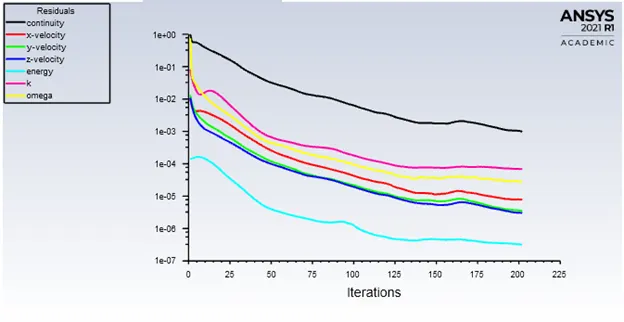
The above plot shows the scaled residuals over the iterations.
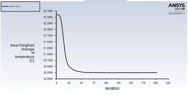
The above plot shows the plot of outlet face temperature over the iterations.
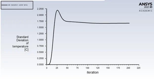
The above plot shows the plot for a standard deviation for the outlet temperature over the iterations.
Following are the plots and results of the test case:
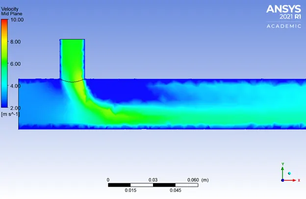
The above diagram shows the contour plot for the velocity at the mid-plane.
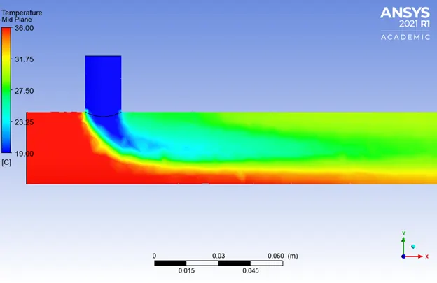
The above diagram shows the contour plot for the temperature at the mid-plane.
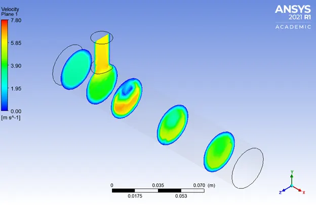
The above diagram shows the contour plot for the velocity at different sections of the pipe.
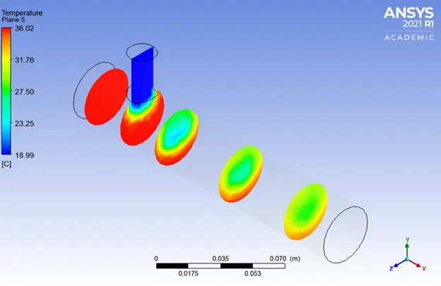
The above diagram shows the contour plot for the temperature at different sections of the pipe.
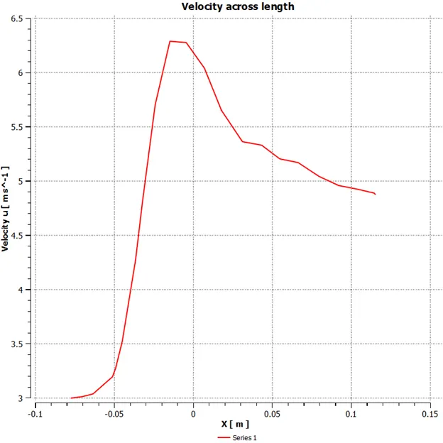
The above diagram shows the line plot for the velocity over the length of the pipe.
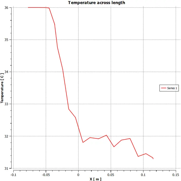
The above diagram shows the line plot for the temperature over the length of the pipe.
The area-weighted average at the outlet face after the convergence was achieved was 30.25 degree Celsius with a standard deviation of 1.66 degree Celsius.
Note on the turbulence model used.
- The exact same mesh with the exact same initial and boundary conditions as the 1st case was used to run the solution with the only difference being the turbulence model which was k-Omega SST instead of k-eplison.
- It is observed that the area-weighted average temperature at the outlet face and its standard deviation are comparable with that of the one obtained using the k-eplison model.
- The number of iterations taken to achieve convergence using the k-omega model is lower compared to the k-eplison.
Therefore, since we get comparable results in a lesser number of iterations using the k-omega SST model the computation time is lesser for the default mesh size of approximately 0.01m, the same turbulence model and the similar element sizing is going to be used for the further cases.
Case 4: Short Mixing Tee with momentum ratio 4.
Note: The mesh size and the number of elements is the same as the 1st case.
The initial velocity and temperature conditions are as follows:
- The velocity at the inlet in the x-direction is 3 m/s and the initial temperature is 36 degrees Celsius.
- The velocity at the inlet in the y-direction is 12 m/s and the initial temperature is 19 degrees Celsius.
The solution was run, and it achieved convergence at 230 iterations. And the following are the different plots obtained in fluent.
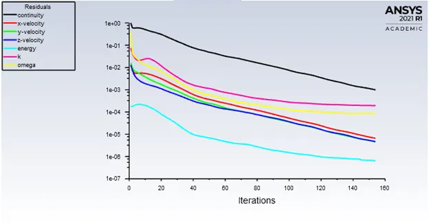
The above plot shows the residuals over the iterations.
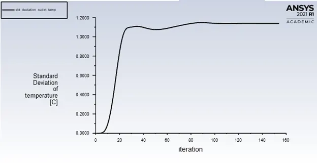
The above plot shows the standard deviation at the outlet face over the iterations.
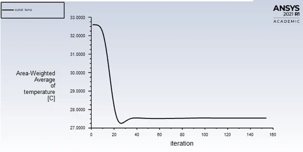
The above plot shows the temperature at the outlet face over the iterations.
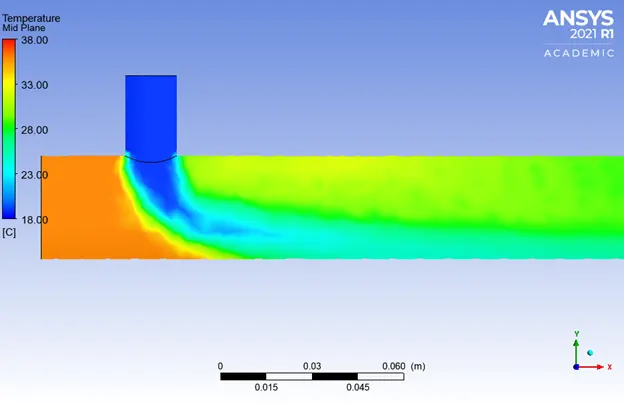
Above is the contour plot of temperature distribution at the midplane.
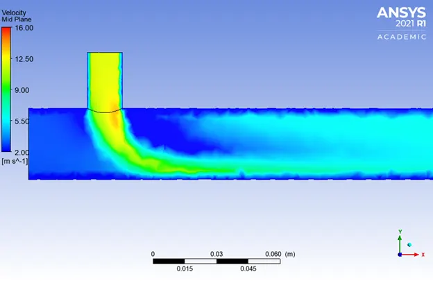
Above is the velocity contour at the mid-plane.
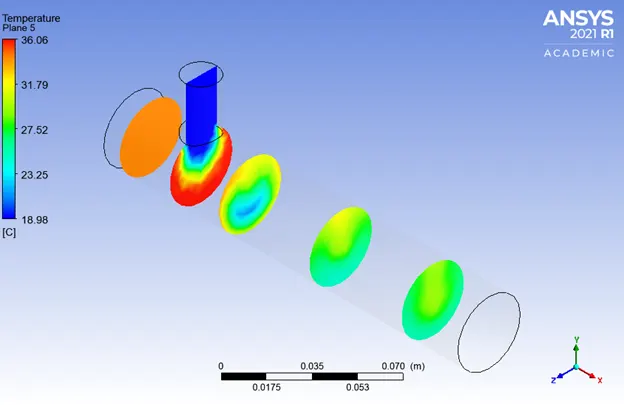
Above is the temperature contour at different sections of the pipe.
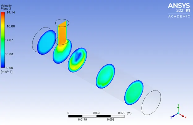
Above is the velocity contour at different sections of the pipe.
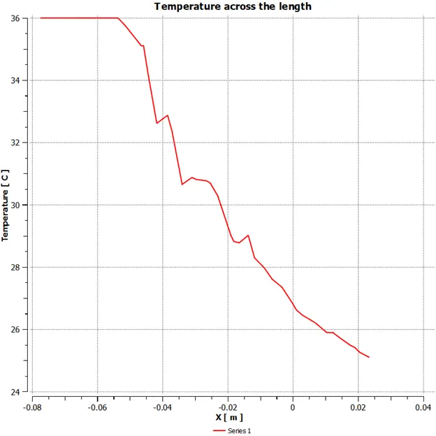
Above is the line plot for temperature variation along the length of the pipe.
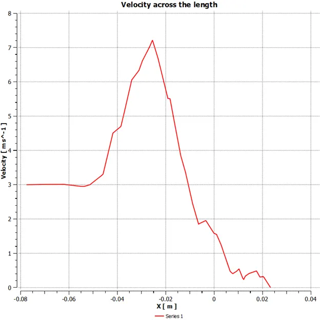
Above is the line plot for the velocity variation across the length of the pipe.
The area-weighted average at the outlet face after the convergence was achieved was 27.54 degree Celsius with a standard deviation of 1.14 degree Celsius.
Case 5: Long mixing tee with momentum ratio 2.
The mesh quality and statistics are as follows:
|
Element sizing (By default) |
Number of nodes |
Number of elements |
|
0.010219m |
49569 |
267042 |
The views for the mesh are as follows:
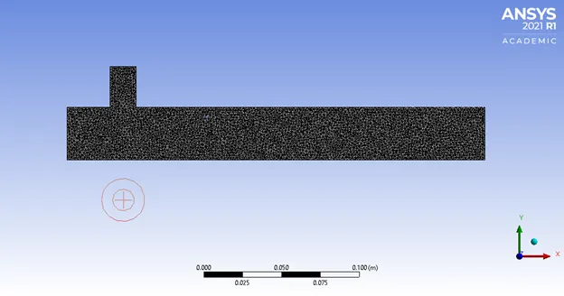
Above is the section plane of the mesh along the middle of xy plane.
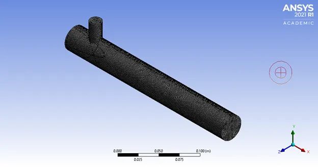
Above is the isometric view of the mesh.
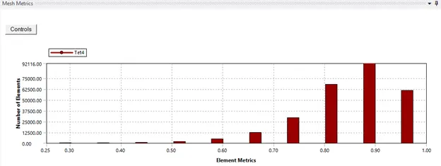
Above is the bar graph of the mesh metrics.
The initial velocity and temperature conditions are as follows:
- The velocity at the inlet in the x-direction is 3 m/s and the initial temperature is 36 degrees Celsius.
- The velocity at the inlet in the y-direction is 6 m/s and the initial temperature is 19 degrees Celsius.
The solution was run, and it achieved convergence at 107 iterations. And the following are the different plots obtained in fluent.
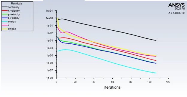
Above is the plot for the residuals over the iterations.
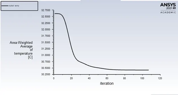
Above is the plot for the outlet temperature at the outlet face over the iterations.
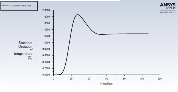
Above is the plot for the standard deviation of the outlet temperature over the iterations.
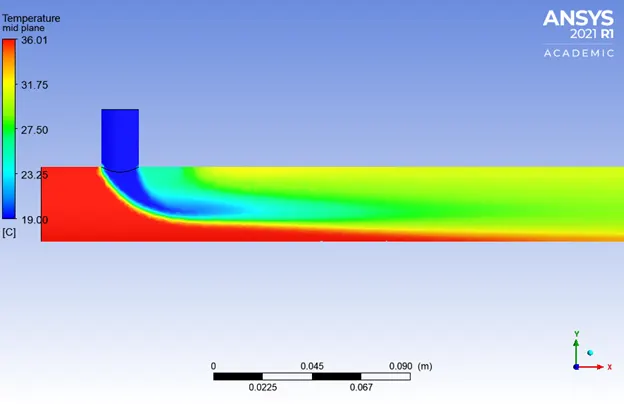
Above is the temperature contour at the midplane.
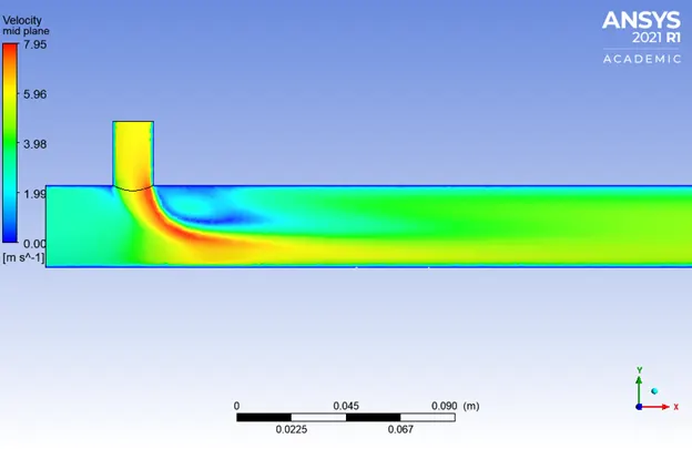
Above is the velocity contour at the mid-plane.
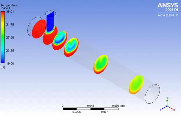
Above are the temperature contours at the different sections of the pipe.
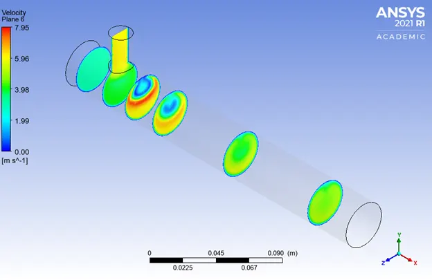
Above is the velocity contour at the different sections of the pipe.
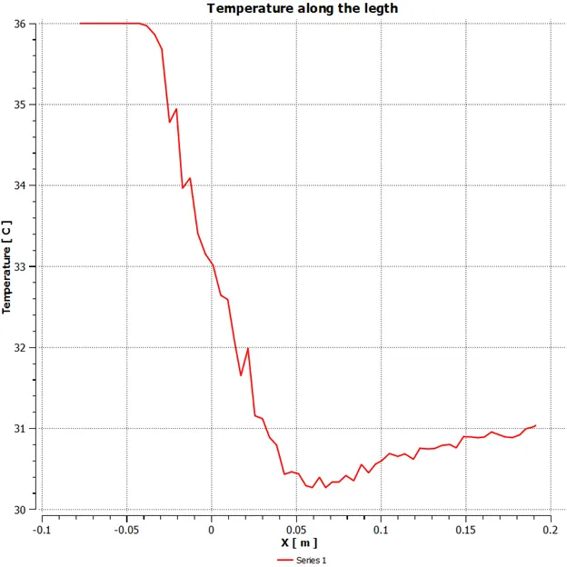
Above is the line plot of the variation in temperature along the length of the pipe.
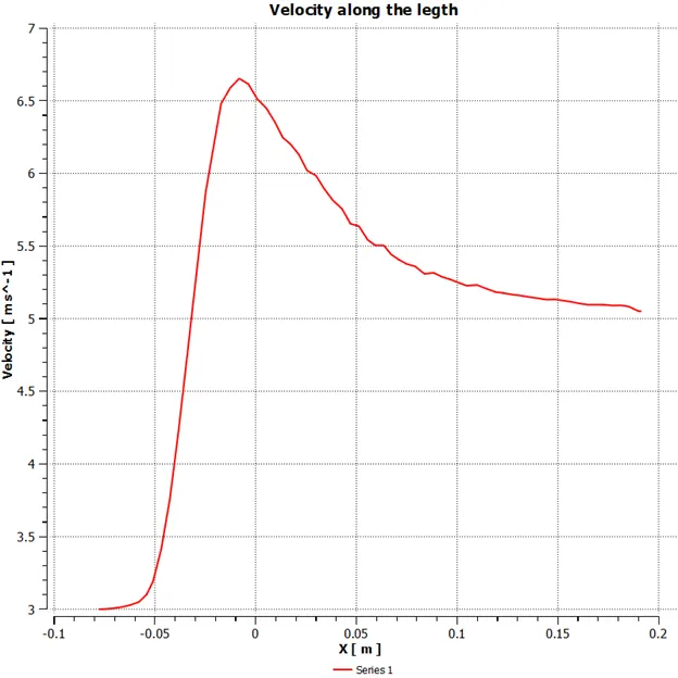
Above is the line plot of the variation of velocity along the length of the pipe.
The area-weighted average at the outlet face after the convergence was achieved was 30.42 degree Celsius with a standard deviation of 1.26 degree Celsius.
Case 6: Long mixing tee with momentum ratio 4.
Note: The exact same mesh which was used to run case 5 is being used to run case 6. Hence, all the mesh metrics and the element sizing are the same as that of case 5.
The initial velocity and temperature conditions are as follows:
- The velocity at the inlet in the x-direction is 3 m/s and the initial temperature is 36 degrees Celsius.
- The velocity at the inlet in the y-direction is 12 m/s and the initial temperature is 19 degrees Celsius.
The solution was run, and it achieved convergence at 128 iterations. And the following are the different plots obtained in fluent.
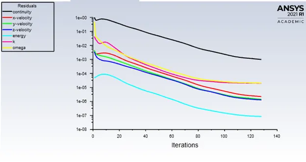
Above is the residuals plot over the iterations.
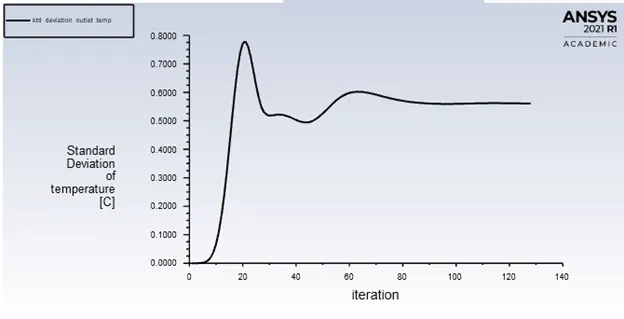
Above is the standard deviation of the temperature at the outlet face over the iterations.
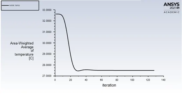
Above is the temperature at the outlet face over the iterations.
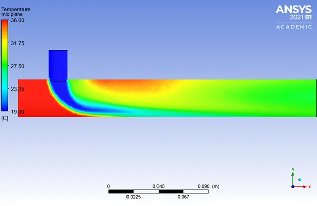
Above is the temperature contour at the mid plane.
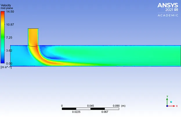
Above is the velocity contour at the mid-plane.
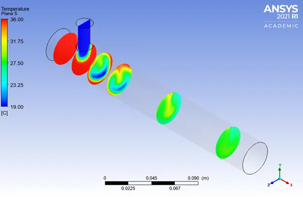
Above is the temperature contour at the different sections of the pipe.
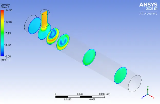
Above is the velocity contour at different sections of the pipe.
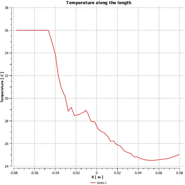
Above is the line plot of the variation in temperature along the length of the pipe.
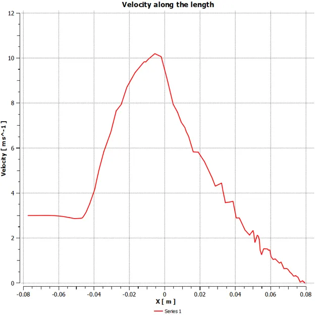
Above is the line plot of the variation in velocity across the length of the pipe.
The area-weighted average at the outlet face after the convergence was achieved was 27.5 degree Celsius with a standard deviation of 0.56 degree Celsius.
The results of the different test cases are tabulated as follows:
| Case no. | Case description | No. of grid elements | Iterations of convergence | Outlet face temp | Std. deviation |
| Case 1 | Short, momentum ratio 2 | 12760 | 230 | 30.21 | 1.62 |
| Case 2 | Short, momentum ratio 2, fine grid | 455917 | 131 | 30.37 | 1.8 |
| Case 3 | Short, momentum ratio 2, k-omega SST | 12760 | 202 | 30.25 | 1.66 |
| Case 4 | Short, momentum ratio 4 | 12760 | 157 | 27.54 | 1.14 |
| Case 5 | Long tee, momentum ratio 2 | 267042 | 107 | 30.42 | 1.26 |
| Case 6 | Long tee, momentum ratio 4 | 267042 | 128 | 27.5 | 0.56 |