A literature review on Finite Volume Method.

Finite Volume Method:

The Finite Volume Method (FVM for short) is used to evaluate elliptic, parabolic, or hyperbolic partial differential equations, based on the conservation laws. Just like the Finite Difference Method (FDM) and the Finite Element Method (FEM), FVM also evaluates the variables at discrete locations of the geometry under consideration as the computational domain. FVM divides the geometry into a finite number of elements (forming a mesh/grid). This mesh could either be structured or unstructured, hence forming a finite number of control volumes in which the governing equations are conserved.

This particular discretization of the domain into a finite number of control volumes can be performed by adopting a vertex-centered approach, where each node of the mesh is the center of the control volume, whose boundaries are obtained by connecting the centroids of each element and the midpoints of each element edge. This is different from the Finite Element Method where the discretization is done in a cell-centered approach, where the control volumes coincide with the nodal points. The following figures show the vertex centered meshing in the FVM:

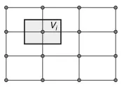
FVM explained through an example of 1D heat conduction phenomenon:

Consider the following diagram:

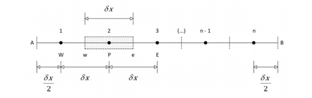
Here, using FVM, the 1D domain is discretized into a finite number of control volumes with nodal points. These nodal points define the space between the boundary points A and B. A general point P is identified and its neighbors on either direction are identified to the W at the right side (west side) of P and E to the left side (East side) of P. The west side face of the control volume is denoted by w and the east side face of the control volume is denoted by e. The distance between the points W and E is `2δx`, and hence the distance between P and either E or W is and the distance between P and either w or e is `δx/2`

The next step in FVM is the integration of the governing equations over a control volume so that it yields a discretized equation at its nodal point P. To arrive at that, let us first look at the 1d steady-state diffusion equation which is given by:

`d/dx (Γ dϕ/dx)+S=0`

Where `Γ` is the diffusion coefficient, `ϕ` is the property of under consideration undergoing diffusion and S is the source term. Now, the integration of this governing equation gives the following:

`∫_(CV)d/dx (Γ dϕ/dx)dV+∫_(CV)SdV = 0`

`=>(ΓA (dϕ)/dx)_e - (ΓA (dϕ)/(dx))_w +S ̅ΔV=0`

Here,

A is the cross-sectional area,

`ΔV` is the volume and

`S ̅` is the average value of the source term in the control volume.

One of the most interesting things about the discretized forms of the FVM is that it gives a very clear physical interpretation. Here, the above equation means, the diffusive flux of `ϕ` leaving the east face minus the diffusive flux of `ϕ` entering the west face is equal to the generation of `ϕ`. It means that the property `ϕ` is conserved within the control volume.

The diffusive fluxes are evaluated using the central differencing as follows:

`(ΓA (dϕ)/(dx))_e=Γ_e A_e ((ϕ_E-ϕ_P)/(δx))`

`(ΓA (dϕ)/(dx))_w=Γ_w A_w ((ϕ_P-ϕ_W)/(δx))`

Here, the `δx` are considered to be uniform (as a case of structured mesh. The case of the unstructured mesh also works equally well by having the appropriate values put at the right places.)

In practical conditions, the source terms are said to be a function of the dependent variable. Hence, we have:

`s ̅Δv=s_u+s_P ϕ_P`

Therefore, when we substitute these equations in our governing equation, we have:

`Γ_e A_e ((ϕ_E-ϕ_p)/(δx))-Γ_w A_w ((ϕ_P-ϕ_w)/(δx))+ s_u+s_P ϕ_P=0`

This can be rearranged and simplified as follows:

`a_P ϕ_P=a_W ϕ_W+a_E ϕ_E+s_u`

Where,

`a_W=Γ_w/(δx)A_w`

`a_E=Γ_e/(δx) A_e`

`a_P=a_w+a_E-s_P`

This equation can be obtained for all the finite number of volumes in our domain of interest and can be arranged and solved for in a matrix form.

Interpolation schemes in FVM: The approximation of surface and volume integrals requires values of the variables at locations other than the defined nodes at the control volume. We can compute the values at these locations using various interpolation schemes. The following are the different interpolation schemes:

Upwind Interpolation Scheme (UDS): Depending on the direction of flow the upwind interpolation scheme is equivalent to calculating either the forward difference or the backward finite difference approximation. It is first-order accurate.

Central Difference Approximation Scheme (CDS): The central difference scheme is equivalent to using the central difference scheme. This interpolation is second-order accurate and may produce oscillatory solutions.

Linear Upwind Difference Scheme (LUDS): The linear upwind interpolation is second-order accurate and is equivalent to the one-sided three-point finite difference approximation.

Quadratic Upwind Interpolation (QUICK): The quadratic upwind interpolation scheme is derived using polynomial fitting. This is third-order accurate but prone to oscillations.

Flux Limiters:

The Flux Limiters are used in high-resolution schemes to avoid oscillations that would otherwise occur with high order spatial discretization schemes due to shocks, discontinuities, or sharp changes in the solution domain. The main idea behind constructing a flux limiter scheme is to limit the spatial derivatives to realistic values. To understand the flux limiter functions better, let us consider the following 1D semi-discrete scheme:

`(du_i)/dt+1/(Δx_i ) [F(u_(i+1/2) )-F(u_(i-1/2) )]=0`

Where `F(u_(i+1/2) )` and `F(u_(i-1/2) )` represent the edge fluxes of the i^th cell.

These fluxes can be represented as low and high resolution schemes and hence the flux limiter can switch between these schemes depending upon the gradients and they are represented as follows:

`f(u_(i+1/2) )=f_(i+1/2)^(low)-ϕ(r_i )-(f_(i+1/2)^(low)- f_(i+1/2)^(high) )`

Here,

f ^low = low resolution flux,

f ^high = high resolution flux,

`ϕ(r)` = flux limiter function

And r represents the ratio of the successive gradients on the solution grid, i.e.,

`r_i=(u_i-u_(i-1))/(u_(i+1)-u)`

The flux limiter is set to be constrained between the values of 0 and 1. Hence, when the limiter is equal to 0, the flux is represented by a low-resolution scheme and when the limiter is equal to 1 the flux is represented by a high-resolution scheme. The following figure shows a limiter function in an r-Ѱ diagram. Where Ѱ is a symmetry-property for limiter functions.

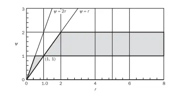
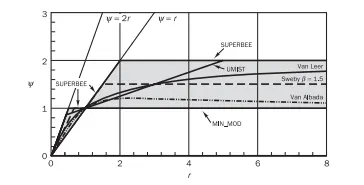
There are various types of flux limiters developed, and no particular limiter is known to work well with all types of problem definitions and hence, the different types of flux limiters are selected on a trial and error basis. The following are some of the most popular flux limiter functions found in literature:

1. Van Leer is described as:

`ϕ(r)=(r+|r|)/(1+|r| )`

2.Van Albada which is described as:

`ϕ(r)=(r^2+r)/(r^1+1)`

3. Min-Mod which is described as:

`ϕ(r)= min⁡(r,1) if r>0; 0 if r>=0`

4. SUPERBEE which is described as:

max[0, min(2r,1), min(r,2)]

5. Sweby which is described as:

max[0, min(βr,1), min(r,β)]

6. QUICK which is described as:

max[0,min(2r, (3+r)/4,2)]

7. UMIST which is described as:

max[0,min(2r, (1+3r)/4, (3+r)/4, 2)]

The following diagram shows the comparison of the various limiter functions:

Key advantages of FVM over FDM:

1. In FVM the discrete conservation laws are conserved.
2. In most cases, one can isolate a single finite volume and apply the conservation law. So, in those cases, cells can be programmed independently.
3. It is much easier to implement FVM in unstructured grids.
4. The formulations in FVM give a much better physical interpretation of the conservation laws.

This concludes a short literature review for the Finite Volume Method.