Rankine Cycle simulator using MATLAB.

Aim: To create a Rankine Cycle simulator in MATLAB.

Objectives:

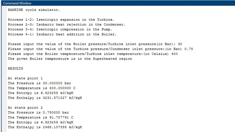
1. The code should calculate the state point variables based on user inputs.
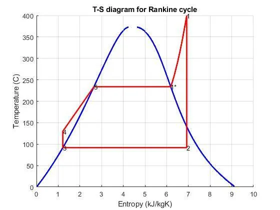
2. To plot the T-S diagram for the Rankine cycle.
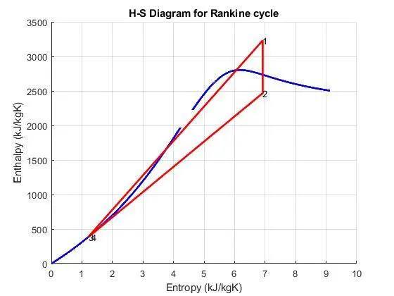
3. To plot the H-S diagram for the Rankine cycle.

Rankine cycle: The Rankine cycle is one of the many thermodynamic cycles whose principles are used to produce mechanical work. Rankine cycle describes the processes that occur in an external combustion engine, more specifically, a steam turbine system that extracts mechanical work out of thermal energy in the steam. The Rankine cycle consists of four major components namely, a Boiler, a Turbine, a Condenser, and a Pump. Each component changes the state and properties of the fluid that moves through it, by adding and removing heat and work, in order to transfer energy from heat to work. A simple schematic diagram that represents the Rankine cycle is as follows:

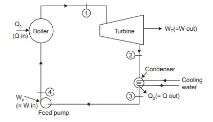
Boiler: It can also be referred to as the Steam Generator. It turns the fluid at room temperature and pressure, to vapour or steam at an extremely high temperature, which is usually termed as “Superheated vapour”.

Turbine: The steam produced in the Boiler is allowed to expand in the Turbine and it extracts mechanical work out of the steam coming in from the Boiler.

Condenser: It operates at a constant pressure where heat is released into the environment, compressing the state of the fluid back down to a liquid-gas mixture, that is mostly liquid. This state is otherwise known as the “Saturated liquid”.

Pump: It pressurizes the saturated liquid back up to the pressure of the turbine by bringing work back into the system, turning to a highly pressurized liquid which is usually referred to as a “Compressed liquid”. The liquid then goes back into the Boiler and the cycle continues.

In order to understand the thermodynamic aspects of the cycle, we need to know the processes involved in the cycle. The Rankine cycle has four processes that are listed below:

Boiler: It can also be referred to as the Steam Generator. It turns the fluid at room temperature and pressure, to vapour or steam at an extremely high temperature, which is usually termed as “Superheated vapour”.

Turbine: The steam produced in the Boiler is allowed to expand in the Turbine and it extracts mechanical work out of the steam coming in from the Boiler.

Condenser: It operates at a constant pressure where heat is released into the environment, compressing the state of the fluid back down to a liquid-gas mixture, that is mostly liquid. This state is otherwise known as the “Saturated liquid”.

Pump: It pressurises the saturated liquid back up to the pressure of the turbine by bringing work back into the system, turning to a highly pressurized liquid which is usually referred to as a “Compressed liquid”. The liquid then goes back into the Boiler and the cycle continues.

In order to understand the thermodynamic aspects of the cycle, we need to know the processes involved in the cycle. The Rankine cycle has four processes that are listed below:

Process 4-1: Isobaric heat addition in the Boiler.

Applying the Steady Flow Energy Equation for Boiler as the control volume, we get:

h₄ + Q₁ = h₁

_⇒ Q₁ = h₁ + h₄

Process 1-2: Isentropic expansion in the turbine.

Applying the Steady Flow Energy Equation for Turbine as the control volume, we get:

h₁ = W_T + h₂ , where W_T is the Turbine work,

⇒ W_T = h₁ – h₂

Process 2-3: Isobaric heat rejection in the Condenser.

Applying the Steady Flow Energy Equation for Condenser as the control volume, we get:

h₂ = Q₂ + h₃

⇒ Q₂ = h₂ – h₃

Process 3-4: Isentropic compression in the Pump.

Applying the Steady Flow Energy Equation for Pump as the control volume, we get:

h₃ + W_P = h₄

⇒ W_P = h₄ - h₃

The net power output of the Rankine cycle is given by:

W_net = W_T - W_P

Therefore, the thermal efficiency of the Rankine cycle will be given by:

η_Rankine = `(W_T-W_p)/Q_1`

In order to plot the T-S and H-S diagrams for the Rankine cycle, the Steam-table needs to be used extensively. Hence, for the program in MATLAB, it is necessary to have the XSteam library in the directory of our code to create the Rankine cycle simulator. The link to the library is as follows:

https://drive.google.com/open?id=1RK_fvrOj38CIaQvmLT1S3daqHnxKCGU-

The MATLAB code for the Rankine cycle simulator is as follows:

%MATLAB code for a Rankine cycle simulator

clear all
close all
clc

%Printing the processes in the Rankine cycle.
fprintf('%s \n \n','RANKINE cycle simulator.');
fprintf('%s \n','Process 1-2: Isentropic expansion in the Turbine.');
fprintf('%s \n','Process 2-3: Isobaric heat rejection in the Condenser.');
fprintf('%s \n','Process 3-4: Isentropic compression in the Pump.');
fprintf('%s \n \n','Process 4-1: Isobaric heat addition in the Boiler.');

%Taking the inputs for the Boiler pressure, Turbine pressure and the Boiler temperature.
p1 = input('Please input the value of the Boiler pressure/Turbine inlet pressure(in Bar): ');
p2 = input('Please input the value of the Turbine pressure/Condenser inlet pressure:(in Bar) ');
t1 = input('Please input the Boiler temperature/Turbine inlet temperature:(in Celsius) ');

%To find if the Boiler temperature is at the saturated region or the superheated region

t_sat = XSteam('Tsat_p', p1);

if t1>t_sat
  t_sup = t1;
  h1 = XSteam('h_pt',p1,t_sup);
  s1 = XSteam('s_pt',p1,t_sup);
  fprintf('%s \n \n','The given Boiler temperature is in the Superheated region');
    
elseif t1 == t_sat;
  h1 = XSteam('hL_p',p1);
  s1 = XSteam('sL_p',p1);
  fprintf('%s \n \n','The given Boiler temperature is the Saturated Liquid Temperature');
  
else
  fprintf('%s \n \n','The given Boiler temperature is lesser than the Satureted Liquid Temperature')
    
end

%Since the process at Turbine is Isentropic expansion, there is no change in Entropy
s2 = s1;

sL1 = XSteam('sL_p',p1);
sV1 = XSteam('sV_p',p1);

sf2 = XSteam('sL_p',p2);
sg2 = XSteam('sV_p',p2);

hf2 = XSteam('hL_p',p2);
hg2 = XSteam('hV_p',p2);

%Calculating the volume fraction.
x2 = (s2-sf2)/(sg2-sf2);

h1 = XSteam('h_pt',p1,t1);
h2 = hf2+(x2*(hg2-hf2));

%At Temperature T2, the medium is neither fully liquid not fully gas, hence T2 is given by:
t2 = XSteam('Tsat_p',p2);

%At the condenser, the medium rejects heat at a constant pressure. Hence we have:
p3 = p2;

t3 = t2;

h3 = XSteam('hL_p',p3);

s3 = XSteam('sL_p',p3);

%At the pump, the medium undergoes isentrophic compression, hence we have:
s4 = s3;

%At the Boiler, the heat is added at a constant pressure. Hence we have:
p4 = p1;

%Since the process is at constant pressure, the Specific Heat Capacity at constant pressure is:
cp = XSteam('Cp_ps',p4,s4); 

%Since the process is at constant volume, the Specific Heat Capacity at constant volume is:
cv = XSteam('Cv_ps',p4,s4);

%We find T4 by assuming the medium obeys the Ideal Gas Law:
gamma = cp/cv;

t4 = t3*(p4/p3)^((gamma-1)/gamma);

vf = XSteam('vL_p',p3);

%Calculating pump work
Wp = vf*(p1-p2)*100;
h4 = Wp + h3;

%Calculating work output from Turbine
Wt = h1 - h2;

%Calculating heat input at the Boiler
q1 = h1 - h4;

%Calculating heat rejected at the Condenser
q2 = h2 - h3;

%Calculating the net work output
W_net = Wt - Wp;

%Calculating thermal efficiency in percentage of the cycle (work output/heat input) 
eta = (W_net/q1)*100;

%Following lines are used to plot the Vapour Dome and the T-S diagram.

temp = linspace(1,373,1000);

for i = 1:length(temp)
  
  hl(i) = XSteam('hL_T',temp(i));
  hv(i) = XSteam('hV_T',temp(i));
  sl(i) = XSteam('sL_T',temp(i));
  sv(i) = XSteam('sV_T',temp(i));
  
end

figure(1)

hold on;

plot(sl,temp,'color','b','linewidth',2);
plot(sv,temp,'color','b','linewidth',2);
xlabel('Entropy (kJ/kgK)');
ylabel('Temperature (C)');
title('T-S diagram for Rankine cycle');
grid on;
plot([s1 s2 s3 s4 sL1 sV1],[t1 t2 t3 t4 t_sat t_sat],'color','r','linewidth',2);

t = linspace(t_sat,t_sup,1000);
for i = 1:length(t)
  
  sp(i) = XSteam('s_pt',p1,t(i));
  
end

plot(sp,t,'color','r','linewidth',2);

text(s1,t1,'1');
text(s2,t2,'2');
text(s3,t3,'3');
text(s4,t4,'4');
text(sV1,t_sat,'1*');
text(sL1,t_sat,'5');

%Following lines of code is used to plot the H-S diagram.

figure(2)

hold on;

plot(sl,hl,'color','b','linewidth',2);
plot(sv,hv,'color','b','linewidth',2);
plot([s1,s2,s3,s4,s1],[h1,h2,h3,h4,h1],'color','r','linewidth',2);
text(s1,h1,'1');
text(s2,h2,'2');
text(s3,h3,'3');
text(s4+0.1,h4+0.1,'4');
grid on;
xlabel('Entropy (kJ/kgK)');
ylabel('Enthalpy (kJ/kgK)');
title('H-S Diagram for Rankine cycle');

%Printing the results of all the calculations
fprintf('%s \n \n','RESULTS');

fprintf('%s \n','At state point 1');
fprintf('%s %f %s \n','The Pressure is',p1,'bar');
fprintf('%s %f %s \n','The Temperature is',t1,'C');
fprintf('%s %f %s \n','The Entropy is',s1,'kJ/kgK');
fprintf('%s %f %s \n \n','The Enthalpy is',h1,'kJ/kgK');

fprintf('%s \n','At state point 2');
fprintf('%s %f %s \n','The Pressure is',p2,'bar');
fprintf('%s %f %s \n','The Temperature is',t2,'C');
fprintf('%s %f %s \n','The Entropy is',s2,'kJ/kgK');
fprintf('%s %f %s \n \n','The Enthalpy is',h2,'kJ/kgK');

fprintf('%s \n','At state point 3');
fprintf('%s %f %s \n','The Pressure is',p3,'bar');
fprintf('%s %f %s \n','The Temperature is',t3,'C');
fprintf('%s %f %s \n','The Entropy is',s3,'kJ/kgK');
fprintf('%s %f %s \n \n','The Enthalpy is',h3,'kJ/kgK');

fprintf('%s \n','At state point 4');
fprintf('%s %f %s \n','The Pressure is',p4,'bar');
fprintf('%s %f %s \n','The Temperature is',t4,'C');
fprintf('%s %f %s \n','The Entropy is',s4,'kJ/kgK');
fprintf('%s %f %s \n \n','The Enthalpy is',h4,'kJ/kgK');

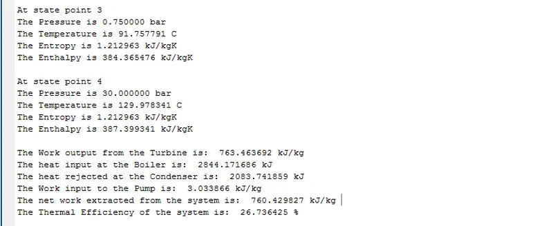
fprintf('%s %f %s \n','The Work output from the Turbine is: ',Wt,'kJ/kg');
fprintf('%s %f %s \n','The heat input at the Boiler is: ',q1,'kJ');
fprintf('%s %f %s \n','The heat rejected at the Condenser is: ',q2,'kJ');
fprintf('%s %f %s \n','The Work input to the Pump is: ',Wp,'kJ/kg');
fprintf('%s %f %s \n','The net work extracted from the system is: ',W_net,'kJ/kg');
fprintf('%s %f %s \n \n','The Thermal Efficiency of the system is: ',eta,'%');

The plots and results for the above code are as follows:

This concludes the project to create a Rankine cycle simulator in MATLAB.